CFD Study on the Influence of Atmospheric Stability on Near-field Pollutant Dispersion from Rooftop Emissions
Abstract
The aim of this work is to investigate the effect of atmospheric stability on near-field pollutant dispersion from rooftop emissions of a single cubic building using computational fluid dynamics (CFD). This paper used the shear stress transport (here after SST) k-ω model for predicting the flow and pollutant dispersion around an isolated cubic building. CFD simulations were performed with two emission rates and six atmospheric stability conditions. The results of the simulations were compared with the data from wind tunnel experiments and the result of simulations obtained by previous studies in neutral atmospheric condition. The results indicate that the reattachment length on the roof (XR) obtained by computations show good agreement with the experimental results. However, the reattachment length of the rooftop of the building (XF) is greatly overestimated compared to the findings of wind tunnel test. The result also shows that the general distribution of dimensionless concentration given by SST k-ω at the side and leeward wall surfaces is similar to that of the experiment. In unstable conditions, the length of the rooftop cavity was decreased. In stable conditions, the horizontal velocity in the lower part around the building was increased and the vertical velocity around the building was decreased. Stratification increased the horizontal cavity length and width near surface and unstable stratification decreased the horizontal cavity length and width near surface. Maintained stability increases the lateral spread of the plume on the leeward surface. The concentration levels close to the ground’s surface under stable conditions were higher than under unstable and neutral conditions.
Keywords:
CFD simulation, SST k-ω model, Isolated building, Rooftop emission, Atmospheric stability1. INTRODUCTION
The dispersion of pollution gives rise to important environmental problems that affect human health and well-being. In urban areas, several potentially unpleasant and dangerous sources of pollution include windblown dust, vehicle exhaust, and the toxins and pollutants emitted from building vents (ASHRAE, 2007). Of these, the pollutant emissions from rooftop vents are a factor that can affect the quality of fresh-air at intakes of the emitting and/or surrounding buildings, and potentially deteriorate the wellbeing of these buildings’ occupants (Lateb et al., 2016).
Many parameters have an effect on the dispersion of gaseous emissions in an urban area, including atmospheric stability, vent height and locations, wind velocity and direction, the height and geometry of the building and exhaust momentum. In terms of the vent locations and atmospheric stability, it is known that the vent locations and stability conditions are the most important factors in the dispersion of pollutant around buildings (Yassin, 2013).
The effect of atmospheric stability on pollutant dispersion in an urban environment has been considered in numerous studies. Higson et al. (1995) investigated dispersion in the building wake under neutral or slightly unstable weather conditions in flat terrain using a model building. Mavroidis et al. (1999) studied the detrainment behavior of contaminants in the wake of an isolated building in the field under atmospheric stability conditions ranging from very stable to very unstable. Uehara et al. (2000) examined the effects of thermal stratification on flow in and above urban street canyons using a wind tunnel. Yassin et al. (2005) investigated pollutant dispersion over a built-up area, in the field and in a wind tunnel, in different thermal stabilities and wind directions. Yassin (2013) recently investigated pollutant dispersion with wind tunnel studies. Yassin (2013) focused on the effect of thermal stability on flow and dispersion of rooftop emissions in the wake region behind a building. He also used Bulk Richardson number for atmospheric stability condition. Santos et al. (2009) used a k-ε model to investigate the effect of the atmospheric stratification on flow and dispersion around an isolated cubical building. They simulated only three stability conditions, namely neutral (LMO=∞, where LMO is Monin-Obukhov Length), stable (LMO=1.2) and unstable (LMO=- 7.0). Therefore, further studies in various stability conditions are needed.
Although much of the prior research has examined pollutant dispersion under various stability conditions, very few CFD studies have dealt with the effect of atmospheric stability on pollutant dispersion near the surface of an isolated building. There is also little work examining the effect of thermal stratification on air pollutant dispersion of rooftop vent emissions. Consequently, there is a need for further study of the effect of thermal stability on pollutant dispersion around a building from rooftop vent emissions. Therefore, this study presents the effect of atmospheric stability on pollutant dispersion around an isolated building using CFD.
2. MATERIALS AND METHODS
2. 1 Numerical Methods
The Fluent CFD software package (Fluent, 2012) was used to simulate wind flow and pollutant dispersion around a cubic building. Reynolds-averaged conservation equations for mass and momentum were used to simulate the processes of interest. Mass and momentum conservation equations are written as follows;
| (1) |
| (2) |
where uj is the velocity of j component, t is the time, xj is the j coordinate, ρ is the air density, μ is the dynamic viscosity; gi is the gravitational body force.
The SST k-ω model is selected for closure of the system of equations composed of the continuity equation and the Reynolds-Averaged Navier-Stokes (RANS) equations. The SST k-ω model of the Fluent software uses two different transport equations to express the turbulence kinetic energy (TKE) k and the specific dissipation rate ω. The SST k-ω accounts for the principal turbulent shear stress and uses across-diffusion term in the ω equation to blend both the k-ω and k-ε models and to ensure that the model equations behave appropriately in both the near-wall and far-field zones. Thus, the SST k-ω model offers superior simulation performance compared with the individual k-ω and k-ε models (Menter et al., 2003).
The SST k-ω model has the following two transport equations (Fluent ver. 14, 2012):
| (3) |
and
| (4) |
In these equations, represents the generation of turbulence kinetic energy due to mean velocity gradients, Gω represents the generation of ω, and Γk and Γω represent the effective diffusivity of k and ω, respectively. Yk and Yω represent the dissipation of k and ω due to turbulence. Dω represents the cross-diffusion term. Sk and Sω are user-defined source terms.
The pollutant dispersion patterns were analyzed after solving the species transport equation in conjunction with the turbulence model equations. The advection–diffusion (AD) module was applied to study the species transport process by analyzing the mass fraction of pollutants in the mixture. Fluent analyzes the mass diffusion process based on the following equations:
| (5) |
Where Ji is the diffusion flux of the species i (kgㆍm-2ㆍs-1);
| (6) |
In these equations, ρ is the density of the mixture (kgㆍm-3), Di,m is the mass diffusion coefficient of the pollutant in the mixture (m2ㆍs-1), DT,i is the thermal diffusion coefficient (m2ㆍs-1), Yi is the mass fraction of the species i (kgㆍkg-1), μt is the turbulent viscosity (kg·m-1ㆍs-1). Turbulent Schmidt number Sct was specified as 0.1 in this study.
2. 2 Computational Domain and Boundary Conditions
The computational domain and boundary conditions are shown in Fig. 1. Dimensions of computational domains are equal to 25H×11H×6H (H=10 m is building height) in the streamwise (x), lateral (z) and vertical (y) directions, respectively. These values were selected by following the COST Action 732 (Franke et al., 2007) and AIJ (Tominaga et al., 2008) guidelines to limit the deterioration of the prescribed inflow profiles along the empty fetch upstream of the building.

Computational domain and boundary conditions
The inlet velocity profile of the horizontal wind velocity is defined (Pieterse and Harms, 2013) as:
| (7) |
where , z(m) is height from the surface. LMO is Monin-Obukhov length. The friction velocity u∗ = 0.3 mㆍs-1 and roughness length z0 = 0.13 m were used in this study.
As illustrated by Lin et al. (2007) the vertical profile of temperature can be defined as follows:
| (8) |
where, T(z) is the air temperature (K) at , zs (1.35 m) is a height above the earth’s surface, ϒd (0.01 Kㆍm-1) is the dry adiabatic lapse rate of Ts, (K) is the air temperature at zs and g (9.8 mㆍs-2) is the gravitational acceleration constant.
The profile of k for thermally stratified atmospheric boundary layers (Pieterse and Harms, 2013) is:
| (9) |
The turbulent dissipation of inlet (Pieterse and Harms, 2013) is defined as follows:
| (10) |
When using a commercial CFD code, Blocken et al. (2007) provide the wall boundary condition by deriving a relationship which brings the rough wall functions in equilibrium with the inlet profiles. For Fluent this relation is given by:
| (11) |
Where ks is the roughness height and Cs is a roughness constant required for the wall function. Roughness height should be smaller than the height of the center point of the wall adjacent cell (=0.25 m) and was consequently set to 0.19 m in this study. The resulting value for Cs is 6.7 is defined through a User Defined Function. At the ground surface, the non-slip condition and zero heat flux are assumed.
2. 3 Simulation Plan
Twelve simulations were designed to test the effect of atmospheric stability on plume dispersion. Two emission velocities are used in this study. To compare the profile of velocity and streamline, emission velocity 0 ms-1 was used. Hydrogen sulfide was selected as a pollutant. Emission velocity 0.619 ms-1 was used to simulate the concentration field of wind tunnel results. As shown in Table 1, six atmospheric stabilities are selected using the Monin-Obukhov length scale LMO. The simulated flow and concentration results of neutral stability condition (D) were compared with the wind tunnel experiments.

Simulation plan to test the effect of atmospheric stability conditions.
3. RESULTS AND DISCUSSION
3. 1 Grid Sensitivity Study
To test grid sensitivity, three grids with cubical cells of 1.0, 0.5 and 0.4 m around building surfaces were used in this study. Franke et al. (2004) recommend the use of hexahedral cells over tetrahedral cells, as hexahedral cells yield smaller truncation errors and better iterative convergence. Therefore, this study selected hexahedral cells. Franke et al. (2004) also recommend keeping the stretching ratio below 1.3 in regions of high gradients, to limit the truncation error. Thus, outside the building block array an expansion ratio of 1.1 was applied. Fig. 2 shows the results of the grid sensitivity study that presents the comparison of the mean horizontal wind velocity U along vertical profiles at two locations with different flow regimes. The first profile (Fig. 2(a)) was located upstream (X/H=-1.0) of cubic building. The second velocity profile (Fig. 2(b)) was located in the leeward wake region (X/H=3.0). As shown in Fig. 2, the profiles show some grid dependency, which becomes smaller on the finer grids. For both locations, very little quantitative differences are present between the 0.4 m-grid and the 0.5 m-grid, whereas for the 1.0 m-grid, even qualitative differences are found in comparison to the 0.5 m-grid. This suggests the 0.5 m-grid with a cell is appropriate for reliably predicting flows around an isolated cubic building. The details of grid sensitivity study can also be found in Jeong (2017). The 0.5 m-grid was modeled around H2S outlet in this study.

Mean wind velocities U (m/s) on different grids at X/H=-1.0 (a) and X/H=3.0 (b), Δ is mesh size, H (=10 m) is building height.
3. 2 Comparison with Wind Tunnel Results
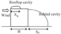
Table 2 compares the reattachment lengths on the roof (XR) and behind the building (XF). The XR values obtained by computations show good agreement with the experimental values. However, XF is greatly overestimated in the simulation result. These results are similar to those shown in a previous study using Realizable k-ε model (Tominaga and Stathopoulos, 2010).
Comparison of reattachment lengths on roof and behind cube of stability D.
Fig. 3 shows profiles of streamwise velocities on the roof and behind the cube at the centerline obtained by the SST k-ω model and the experiment. In this figure, the experimental data for the flows around the cube without vent emission provided by Castro and Robins (1977) is compared with the CFD result for the validation. The differences between the velocity distributions of the experiment and present CFD were rather small.

Comparison of vertical distribution of streamwise velocity on (a) roof center (X/H=0.5) and (b) behind cube (X/H=1.5) at centerline.
Fig. 4 shows the contours of the time-averaged dimensionless concentration, K, on the roof and wall surfaces obtained from the SST k-ω model and the experiment by Li and Meroney (1983). In this study, the experimental and the numerical results presented as dimensionless concentration were as follows:
| (12) |

Distribution of dimensionless concentration K on roof and wall surfaces.
where C is the mass fraction of the tracer gas, L the size of the cube (m), UH is mean wind speed at roof height (ms-1) and Qe the emission rate of the pollutant (m3 s-1).
The concentration of the high concentration region (K>50) upwind of the vent in the experiment was larger than those in SST k-ω on the roof surface. The results of K in SST k-ω model showed a spread smaller than those of the experiment in the downstream direction. However, the concentrations are widely expanded in the horizontal direction in SST k-ω. The general distribution of K given by SST k-ω at the side and leeward wall surfaces is similar to that of the experiment, although the SST k-ω result tends to be a little diffusive. The concentrations at the side wall in the SST k-ω are mainly coming from the roof, as in the experiment.
3. 3 Effect of Atmospheric Stability on Flow Field
In order to evaluate the effect of the atmospheric stability on the flow field behind the building, the x-velocity and streamline of centerline under various atmospheric stabilities are shown in Fig. 5. Generally, reattachment length behind the building was increased in stable conditions compared to in unstable conditions. This means that the mixing effect near the cube under unstable conditions was stronger than in stable conditions.

Velocity and streamline at Z=0 m for six stability conditions
To compare the rooftop cavity, Fig. 6 shows velocity and streamline at Z=0 m to illustrate the reattachment distance for various stability conditions. The result showed that the unstable condition (stability A, B, C) decreased the length of the rooftop cavity. This is because the vertical velocity is increased and the longitudinal velocity decreased around the rooftop of the building. The stable condition (Stability E, F) increased the horizontal velocity in the lower part around the building and decreased the vertical velocity around the building.

Velocity and streamline around building top of centerline (Z=0 m).
In order to compare the temperature distribution around a building for six stability conditions, temperature contours around a building are illustrated in Fig. 7. This comparative view of results illustrates typical temperature profiles in the vertical direction for all boundary layers. However, in strong stable and unstable conditions, the near surface temperature along x direction was slightly changed from inlet conditions. The reason for such results is deemed to be partly because of the use of zero heat flux at the ground surface.

Temperature distribution and streamlines around building.
Fig. 8 illustrates the velocity and streamline at Y=1 m for six stability conditions. Stratification increases the horizontal cavity length and width near the surface. However, unstable stratification decreases horizontal cavity length and width near the surface. This means a stable stability condition will increase horizontal pollutant dispersion compared to an unstable stability condition.

Velocity and streamline at Y=1 m for six stability conditions.
3. 4 Effect of Atmospheric Stability on Concentration Field
Fig. 9 show mass fraction contours for various stability conditions to compare the plume length. As shown in Fig. 9, stratification increases the plume length and results in a larger pollution impact region at leeward facet. However, more pollutants move to the side facet of the building in an unstable stability condition. Although stable stratification suppresses vertical motion and reduces vertical spreading, it also increases lateral motion. As a result, stable stability increases the lateral spread of the plume on the leeward surface. The concentration levels close to the ground surface were higher under stable conditions than under unstable and neutral conditions. This is because the lateral flow carries the contaminant away from the building.

Mass fraction contour of surface for various stability conditions.
Fig. 10 shows the plume contours at Z=0 m for six stability conditions. Unstable stratification decreases horizontal plume length but increases vertical plume height. However, stratification increases the horizontal plume length and decreases vertical plume height. This means a stable stability condition will increase horizontal pollutant dispersion compared to an unstable stability condition.

Centerline plume contours for various stability conditions.
4. CONCLUSIONS
The objective of the paper was to investigate the effect of atmospheric stability on near-field pollutant dispersion from rooftop pollutant emissions, and this was carried out using computational fluid dynamics (CFD). The simulations produced the following conclusions:
- (1) The reattachment length on the roof (XR) obtained by computations show good agreement with the experimental results under neutral stability conditions. However, the reattachment length on the building (XF) rooftop in the simulation is greatly overestimated compared to the wind tunnel result.
- (2) The general distribution of dimensionless K given by SST k-ω at the side and leeward wall surfaces is similar to that of the experiment, although the SST k-ω result tends to be somewhat diffusive.
- (3) The unstable condition (stability A, B, C) decreased the length of the rooftop cavity. The stable condition (Stability E, F) increased the horizontal velocity in the lower part around the building and decreased the vertical velocity around the building.
- (4) Stratification increased the horizontal cavity length and width near the surface, and unstable stratification decreased the horizontal cavity length and width near the surface.
- (5) Stable stability increased the lateral spread of the plume on the leeward surface. The concentration levels close to the ground surface were higher under stable conditions than under unstable and neutral conditions.
Acknowledgments
This work was supported by Kyonggi University Research Grant 2016.
References
- ASHRAE, (2007), Building Air Intake and Exhaust Design. ASHRAE Handbook-Heating, Ventilating, and Air-conditioning Applications (Chapter 44), American Society of Heating, Refrigerating and Air-conditioning Engineers, Atlanta, United States.
-
Blocken, B., Stathopoulos, T., Carmeliet, J., (2007), CFD simulation of the atmospheric boundary layer: wall function problems, Atmospheric Environment, 41, p238-252.
[https://doi.org/10.1016/j.atmosenv.2006.08.019]

-
Castro, I.P., Robins, A.G., (1977), The flow around a surface-mounted cube in uniform and turbulent streams, Journal of Fluid Mechanics, 79, p307-335.
[https://doi.org/10.1017/s0022112077000172]
- FLUENT Ver.14.0, (2012), User’s Guide.
- Franke, J., Hellsten, A., Schlünzen, H., Carissimo, B., (2007), Best practice guideline for the CFD simulation of flows in the urban environment, COST Action 732.
- Franke, J., Hirsch, C., Jensen, A.G., Krüs, H.W., Schatzmann, M., Westbury, P.S., Miles, S.D., Wisse, J.A., Wright, N.G., (2004), Recommendations on the use of CFD in wind engineering, In: van Beeck, J.P.A.J. (Ed.), Proceedings of the international conference on urban wind engineering and building aerodynamics, COST action C14, impact of wind and storm on city life built environment Von Karman Institute, Sint-Genesius-Rode, Belgium, 5-7 May 2004.
-
Higson, H.L., Griffiths, R.F., Jones, C.D., Biltoft, C., (1995), Effect of atmospheric stability on concentration fluctuations and wake retention times for dispersion in the vicinity of an isolated building, Environmetrics, 6, p571-581.
[https://doi.org/10.1002/env.3170060604]
- Jeong, S.J., (2017), A CFD study of near-field odor dispersion around a cubic building from rooftop emissions.
-
Lateb, M., Meroney, R.N., Yataghene, M., Fellouah, H., Saleh, F., Boufadel, M.C., (2016), On the use of numerical modelling for near-field pollutant dispersion in urban environments - A review, Environmental Pollution, 208, p271-283.
[https://doi.org/10.1016/j.envpol.2015.07.039]
- Li, W., Meroney, R.M., (1983), Gas dispersion near a cubical model building - Part I, Mean concentration measurements. Journal of Wind Engineering and Industrial Aerodynamics, 12, p15-33.
- Lin, X.J., Barrington, S., Choiniere, D., Prasher, S., (2007), Simulation of the effect of windbreaks on odour dispersion using the CFD SST k-ω model, Biosystems Engineering, 98, p347-363.
-
Mavroidis, I., Griffiths, R.F., Jones, C.D., Biltoft, C., (1999), Experimental investigation of the residence of contaminants in the wake of an obstacle under different stability conditions, Atmospheric Environment, 33, p939-949.
[https://doi.org/10.1016/s1352-2310(98)00219-2]
- Menter, F.R., Kuntz, M., Langtry, R., (2003), Ten years of industrial experience with the SST turbulence model, In: Hanjalic, K., Nagano, Y., Tummers, M. (Eds.), Turbulence, Heat and Mass Transfer 4, Begell House Inc., Redding, CT, USA, p625-632.
-
Pieterse, J.E., Harms, T.M., (2013), CFD investigation of the atmospheric boundary layer under different thermal stability conditions, Journal of Wind Engineering and Industrial Aerodynamics, 121, p82-97.
[https://doi.org/10.1016/j.jweia.2013.07.014]
-
Santos, J.M., Reis Jr., N.C., Goulart, E.V., Mavroidis, I., (2009), Numerical simulation of flow and dispersion around an isolated cubical building: The effect of the atmospheric stratification, Atmospheric Environment, 43, p5484-5492.
[https://doi.org/10.1016/j.atmosenv.2009.07.020]
-
Tominaga, Y., Mochida, A., Yoshie, R., Kataoka, H., Nozu, T., Yoshikawa, M., Shirasawa, T., (2008), AIJ guidelines for practical applications of CFD to pedestrian wind environment around buildings, Journal of Wind Engineering and Industrial Aerodynamics, 96, p1749-1761.
[https://doi.org/10.1016/j.jweia.2008.02.058]
-
Tominaga, Y., Stathopoulos, T., (2010), Numerical simulation of dispersion around an isolated cubic building: Model evaluation of RANS and LES, Building and Environment, 45, p2231-2239.
[https://doi.org/10.1016/j.buildenv.2010.04.004]
-
Uehara, K., Murakami, S., Oikawa, S., Wakamatsu, S., (2000), Wind tunnel experiments on how thermal stratification affects flow in and above urban street canyons, Atmospheric Environment, 34(10), p1553-1562.
[https://doi.org/10.1016/s1352-2310(99)00410-0]
-
Yassin, M.F., (2013), Experimental study on contamination of building exhaust emissions in urban environment under changes of stack locations and atmospheric stability, Energy and Buildings, 62, p68-77.
[https://doi.org/10.1016/j.enbuild.2012.10.061]
-
Yassin, M.F., Kato, S., Ooka, R., Takahashi, T., Kouno, R., (2005), Field and wind-tunnel study of pollutant dispersion in a built-up area under various meteorological conditions, Journal of Wind Engineering and Industrial Aerodynamics, 93, p361-382.
[https://doi.org/10.1016/j.jweia.2005.02.005]