Numerical Simulation of Extreme Air Pollution by Fine Particulate Matter in China in Winter 2013
Abstract
In winter 2013, extreme air pollution by fine particulate matter (PM2.5) in China attracted much public attention. In order to simulate the PM2.5 pollution, the Community Multiscale Air Quality model driven by the Weather Research and Forecasting model was applied to East Asia in a period from 1 January 2013 to 5 February 2013. The model generally reproduced PM2.5 concentration in China with emission data in the year 2006. Therefore, the extreme PM2.5 pollution seems to be mainly attributed to meteorological (weak wind and stable) conditions rather than emission increases in the past several years. The model well simulated temporal and spatial variations in PM2.5 concentrations in Japan as well as China, indicating that the model well captured characteristics of the PM2.5 pollutions in both areas on the windward and leeward sides in East Asia in the study period. In addition, contribution rates of four anthropogenic emission sectors (power generation, industrial, residential and transportation) in China to PM2.5 concentration were estimated by conducting zero-out emission sensitivity runs. Among the four sectors, the residential sector had the highest contribution to PM2.5 concentration. Therefore, the extreme PM2.5 pollution may be also attributed to large emissions from combustion for heating in cold regions in China.
Keywords:
PM2.5, China, Air quality model, WRF/CMAQ, Residential combustion1. INTRODUCTION
Particulate matter (PM) with an aerodynamic diameter less than 2.5 μm(PM2.5) is an atmospheric pollutant that mainly consists of several major components, such as sulfate, nitrate, ammonium, organics and so on. Based on the accumulated epidemiological evidence, the World Health Organization (WHO) issued the air quality guideline for PM2.5, which is 10 μg m-3 as the long-term (annual mean) value and 25 μg m-3 as the short-term (24-hour) value (WHO, 2006).
The rapid growth in economic activity and energy consumption in recent decades has resulted in increased anthropogenic emissions of air pollutants in Asian countries, particularly in China (Zhang et al., 2009; Ohara et al., 2007). A large number of studies have investigated impacts of Asian emissions on the atmospheric environment by using numerical models (e.g., Lin et al., 2010; Fu et al., 2009; Shimadera et al., 2009).
In China, studies on PM2.5 observations have been gradually conducted since 2000 (e.g., Zhao et al., 2013; Zhao et al., 2009; Duan et al., 2006; Zheng et al., 2005). These studies have shown substantially high PM2.5 concentrations in China. Annual mean PM2.5 concentrations at urban sites in Beijing were 100-112 μg m-3 in 2000 (Zheng et al., 2005), 97-107 μg m-3 in 2001-2002 (Duan et al., 2006), 84-94 μg m-3 in 2005-2007 (Zhao et al., 2009) and 123 μg m-3 in 2009-2010 (Zhao et al., 2013). Also in winter 2013, China faced extreme PM2.5 pollution, and hourly PM2.5 concentration reached 886 μg m-3 on 12 January in Beijing (https://twitter.com/BeijingAir). The extreme PM2.5 pollution was widely reported in mass media and attracted much public attention.
In this study, the Community Multiscale Air Quality model (CMAQ) (Byun and Schere, 2006) driven by the Weather Research and Forecasting model (WRF) (Skamarock and Klemp, 2008) was utilized in order to simulate the extreme PM2.5 pollution in China in winter 2013. The model performance was evaluated in both areas on the windward side (China) and the leeward side (Japan) in East Asia. In addition, contribution rates of anthropogenic emission sectors in China to PM2.5 concentrations were estimated by conducting zero-out emission sensitivity runs.
2. METHODOLOGY
2. 1 Numerical Model
This study used the Advanced Research WRF version 3.4.1 and CMAQ version 5.0.1. Fig. 1 shows the modeling domain for CMAQ that covers a wide area of East Asia. The horizontal resolution and the number of grid cells are 64 km and 96×80, respectively. The vertical layers consist of 30 sigma-pressure coordinated layers from the surface to 100 hPa with the middle height of the first layer being approximately 26 m.
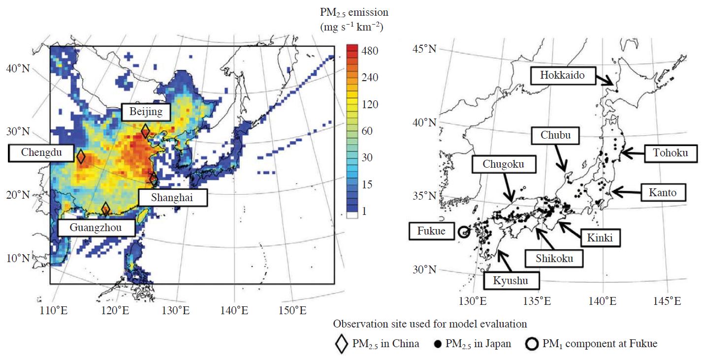
Modeling domain for CMAQ simulation with primary PM2.5 emission rate and locations of observation sites.
The meteorological simulation by WRF was conducted for a period from 28 December 2012 to 5 February 2013. Initial and boundary conditions were derived from the final operational global analysis data and the high-resolution, real-time, global sea surface temperature analysis data of the U.S. National Centers for Environmental Prediction. WRF was configured with the cumulus parameterization of Kain (2004), the planetary boundary layer (PBL) parameterization of Hong et al. (2006), the microphysics scheme of Hong and Lim (2006), the land surface model of Chen and Dudhia (2001), the longwave radiation scheme of Mlawer et al. (1997) and the shortwave radiation scheme of Dudhia (1989). Grid nudging was applied to wind, temperature and humidity with a nudging coefficient of 3.0×10⁻⁴ sec-1 for the entire period.
The air quality simulation by CMAQ was conducted for a period from 1 January 2013 to 5 February 2013 with the hourly WRF results processed by the Meteorology- Chemistry Interface Processor (MCIP) version 4.1. The meteorological data processed with MCIP were also applied to the Hybrid Single Particle Lagrangian Integrated Trajectory model version 4 (Draxler and Hess, 1997) for the backward trajectory analysis. Initial and boundary concentrations were obtained from the Model for Ozone and Related Chemical Tracers version 4 (Emmons et al., 2010). CMAQ was configured with the gas-phase chemical mechanism of Carter (2000), the fifth generation CMAQ aerosol module and the aqueous process option. Fine particles in CMAQ are represented by the two lognormal distributions called the Aitken and accumulation modes. The total mass concentration of particles in the two modes was used as an approximation of PM2.5 concentration.
2. 2 Emission Data
Anthropogenic emissions of sulfur dioxide (SO2), nitrogen oxides (NOX), carbon monoxide, PM and volatile organic compounds in East Asia except Japan were derived from an emission inventory for Asia in the year 2006 to support the Intercontinental Chemical Transport Experiment phase B (INTEX-B) (Zhang et al., 2009) version 1.2. Because of a lack in the INTEX-B emission data, ammonia emissions were derived from the Regional Emission inventory in ASia (REAS) (Ohara et al., 2007) version 1.11. Anthropogenic emissions in Japan were derived from emission inventories for vehicles in the year 2010 (Morikawa et al., 2012) and for the other sectors in the year 2005 (Nakatsuka et al., 2012). Ship emissions were derived from emission inventories developed by the National Maritime Research Institute (NMRI) and by the Ocean Policy Research Foundation (OPRF) (OPRF, 2012). In addition, pre-mission emission inventories for the Arctic Research of the Composition of the Troposphere from Aircraft and Satellites (http://mic.greenresource.cn/arctas_premission) were used to compensate for a shortage in the anthropogenic emission data. Biogenic emissions were estimated with the Model of Emissions of Gases and Aerosols from Nature (Guenther et al., 2006) version 2.04. Volcanic SO2 emissions were obtained from reports of the Japan Meteorological Agency (http://www.seisvol.kishou.go.jp/tokyo/STOCK/monthly_v-act_doc/monthly_vact.htm).
The INTEX-B emission data have four source sectors: power generation, industry, residential and transportation. Because of strong seasonality in residential combustion for heating, this study applied monthly profiles by province in China estimated by Zhang et al. (2007) to the residential sector. No temporal variation was considered in the other three sectors. The total SO2, NOX and primary PM2.5 emissions in the simulation domain are 118.0, 79.7 and 52.7 Gg day-1, respectively. The emissions from power generation, industry, residential and transportation sectors in China are 50.8, 26.5, 17.3 and 0.3 Gg day-1 for SO2, 25.0, 14.6, 6.4 and 13.7 Gg day-1 for NOX, and 4.0, 18.9, 24.8 and 1.1 Gg day-1 for primary PM2.5, respectively. The primary PM2.5 emission from the residential sector is the largest among the four sectors because of its strong seasonality (12.0 Gg day-1 if no seasonality is considered). A horizontal distribution of primary PM2.5 emission rate in each 64-km grid cell is shown in Fig. 1.
In REAS version 2.1 recently updated by Kurokawa et al. (2013) for the year 2000-2008, while NOX and primary PM2.5 emissions increased monotonically from 2000 to 2008 in China, SO2 emission increased monotonically from 2000 to 2006 and then began to decrease. In the Multi-resolution Emission Inventory for China (MEIC) (http://www.meicmodel.org/) for the year 1990-2010, while NOX emission increased monotonically from 2000 to 2010 in China, SO2 and primary PM2.5 emissions increased monotonically from 2000 to 2006 and then began to decrease. Therefore, the INTEX-B data in the year 2006 may overestimate SO2 and underestimate NOX in China in the study period, and the trend of primary PM2.5 emission after 2006 in China seems to be not clear. No annual adjustment was applied to the INTEX-B data because it can be a source of larger uncertainty.
2. 3 Observation Data
Locations of observation sites used for evaluation of the model are shown in Fig. 1. PM2.5 concentrations in China are observed by the U.S embassy in Beijing and consulates in Shanghai, Guangzhou and Chengdu (https://twitter.com/BeijingAir; https://twitter.com/CGShanghaiAir; https://twitter.com/Guangzhou_Air; https://twitter.com/CGChengduAir). PM2.5 concentrations in Japan are available from the Atmospheric Environmental Regional Observation System (http:// soramame.taiki.go.jp/Index.php). Note that the observation data are provisional values. In addition to these data, concentrations of PM1 components were observed at Fukue by using the Aerosol Chemical Speciation Monitor (Aerodyne Research, Inc.) (Ng et al., 2011).
3. RESULTS AND DISCUSSION
1 Model Performance for PM2.5 Concentrations in China
The WRF/CMAQ performance for PM2.5 concentrations in China was evaluated by time series comparisons and statistical measures: the Pearson’s correlation coefficient (r), mean bias (MB), root mean square error (RMSE) and the index of agreement (IA) of Willmott (1981). Because there may be large uncertainties in spatial allocation of the emission data with a coarse horizontal resolution (0.5°×0.5°) in China to the model grid cells, comparisons of the simulated PM2.5 concentrations derived from two kinds of grid cells with the observations are shown in this chapter. The two kinds are G1 that is the grid cell corresponding to each observation site, which is a usual way, and GB that is the grid cell whose values agree with the observed values the best (=highest IA) among those of the grid cell corresponding to each observation site and the surrounding 8 grid cells.
Fig. 2 shows time series comparisons of the observed and simulated daily mean PM2.5 concentrations at the observation sites in China. Table 1 summarizes statistical measures of the model performance for daily mean PM2.5 concentrations. The model approximately simulated day-to-day variation patterns in PM2.5 concentrations, including the buildups in 9-12 and 25-29 January at Beijing. The two high concentration periods are characterized by low wind speeds and stable atmospheric conditions. During the buildups in 9-12 and 25-29 January at Beijing, simulated mean values were respectively 1.2 and 0.9 m s-1 for wind speeds and 86 and 116 m for PBL heights, with nighttime PBL heights being generally 25 m (the middle height of the first layer at Beijing). The PM2.5 concentration levels at Beijing in the two periods were comparable to or higher than that in a heavy pollution episode in 16-19 January 2010 observed by Zhao et al. (2013). In addition to temporal variations, the model approximately captured the difference in concentration levels among the observation sites. The simulated PM2.5 concentrations of GB at Beijing and Shanghai particularly better agreed with the observed values than those of G1. The two sites are located at the edge of large emission area in Central East China (Fig. 1). Overall, the extreme PM2.5 pollution in China in winter 2013 was generally reproduced by the existing model and input data. The PM2.5 pollution seems to be mainly attributed to meteorological conditions rather than emission increases in the past several years because the model well simulated it by using the INTEX-B emission data in the year 2006. Furthermore, Uno et al. (2013) analysed the relationship between meteorological conditions and PM2.5 concentration over Central East China for Januaries of 2004-2013 with the GEOS-Chem model (Bey et al., 2001) and REAS version 2.1. They found that the Siberian high intensity was exceptionally weak in January 2013, which caused low wind speeds and stable atmospheric conditions. As a result, the extreme PM2.5 pollution occurred in China in winter 2013.
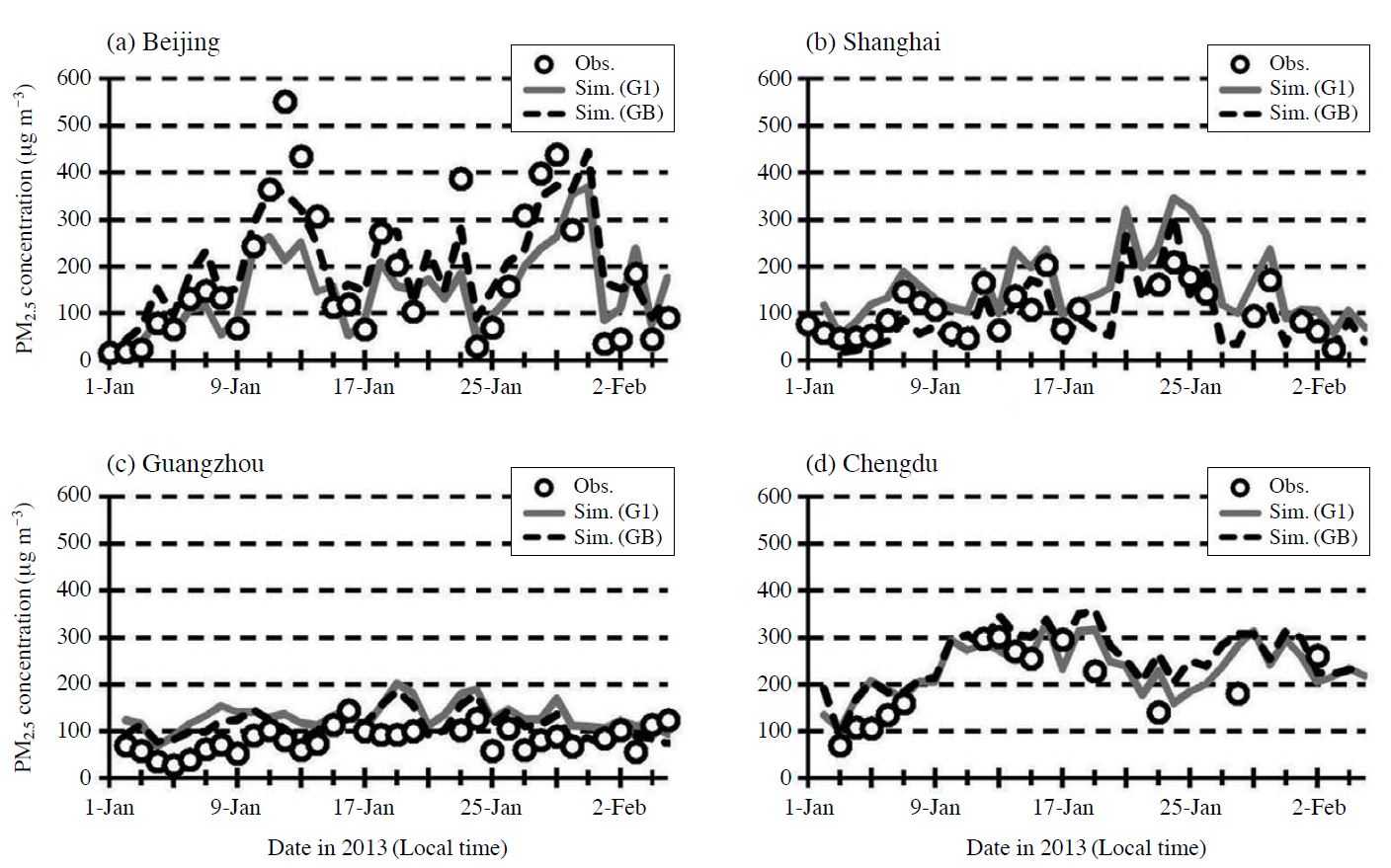
Time series of observed and simulated daily mean PM2.5 concentrations at (a) Beijing, (b) Shanghai, (c) Guangzhou and (d) Chengdu. All dates are in CST (UTC+8). For the simulations, G1 shows values at the grid cell corresponding to each observation site, and GB shows values at the grid cell that agree with the observed values the best among those at the grid cell corresponding to each observation site and the surrounding 8 grid cells.
3. 2 Model Performance for PM2.5 Concentrations in Japan
The WRF/CMAQ performance for PM2.5 concentrations in Japan was evaluated by time series comparisons and the statistical measures by region (Fig. 1). Fig. 3 shows time series comparisons of the observed and simulated daily mean PM2.5 concentrations in Kyushu, Kinki, Kanto and Tohoku. Table 2 summarizes statistical measures of the model performance for daily mean PM2.5 concentrations. The PM2.5 concentration levels in Japan were much lower than those in China. While the model tended to underestimate the PM2.5 concentration levels in Japan, it simulated day-to-day variation patterns in PM2.5 concentrations in Japan as well as China. In both the observation and simulation, the PM2.5 concentration levels tended to be higher in the western regions and lower in the eastern regions. Overall, the model well captured characteristics of the PM2.5 pollutions in both areas on the windward and leeward sides in East Asia.
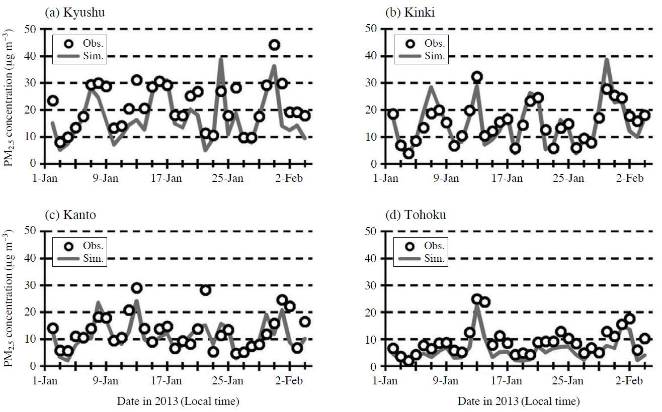
Time series of observed and simulated daily mean PM2.5 concentrations in (a) Kyushu, (b) Kinki, (c) Kanto and (d) Tohoku. All dates are in JST (UTC+9).
3. 3 Model Performance for Concentrations of PM Components
The WRF/CMAQ performance for sulfate, nitrate, ammonium and organics was evaluated by time series comparisons and the statistical measures. Fig. 4 shows time series comparisons of the observed and simulated daily mean concentrations of the four components at Fukue. Table 3 summarizes statistical measures of the model performance for daily mean concentrations of the four components. Note that the observed values are for PM1 and the simulated values are for the approximation of PM2.5. The model simulated day-to-day variation patterns in concentrations of the components at Fukue as well as PM2.5 in Kyushu. However, the model clearly overestimated nitrate, and tended to overestimate ammonium and underestimate sulfate and organics. In earlier literatures, CMAQ tended to underestimate sulfate in winter while the model well captured the concentration level in the other seasons (Shimadera et al., 2011); the model overestimated ammonium nitrate and underestimated organics (Shimadera et al., 2014; Shimadera et al., 2012). Therefore, CMAQ still needs to be revised for better representation of individual PM2.5 components.
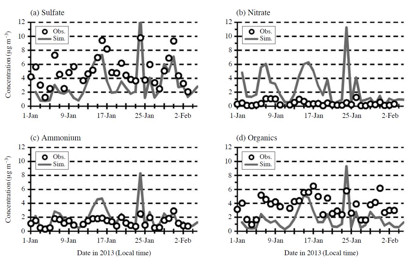
Time series of observed and simulated daily mean concentrations of (a) sulfate, (b) nitrate, (c) ammonium and (d) organics at Fukue. All dates are in JST (UTC+9).
3. 4 Horizontal Distribution of PM2.5
Fig. 5 shows horizontal distributions of the simulated mean PM2.5 concentration in the entire simulation period and PM2.5 concentrations with horizontal wind vectors at the first layer and backward trajectories arriving at 300 m above Beijing and Fukue at specific times. The simulated PM2.5 concentrations were generally higher in and around areas with large primary PM2.5 emissions (Fig. 1). Zhao et al. (2013) showed that PM2.5 pollution in Shijiazhuang, which is located about 280 km southwest of Beijing, was more serious than Beijing. Fig. 5a is consistent with the observation study by Zhao et al. (2013). Fig. 5b explains the buildup of PM2.5 concentration in 9-12 January at Beijing (Fig. 2a). The backward trajectory arriving at Beijing indicates local air pollutants were accumulated for several days under low wind speeds and stable atmospheric conditions. The buildup of PM2.5 concentration in 25-29 January at Beijing (Fig. 2a) also occurred in the similar way. On the other hand, PM2.5 produced in the Asian Continent was sometimes transported over the Northwestern Pacific Ocean by strong northwesterly monsoon (Fig. 5c) or by eastward traveling high pressure systems (Fig. 5d). Fig. 5c indicates that northwesterly monsoon caused the decrease in PM2.5 concentration at Beijing (Fig. 2a), the increase at Shanghai (Fig. 2b) and the increase in Kyushu (Figs. 3a and 4) on 24 January. Fig. 5d indicates that a combination of longrange transport from the Asian Continent and local circulation by a traveling high pressure system increased PM2.5 concentration from 30 January to 1 February in Japan (Fig. 3).
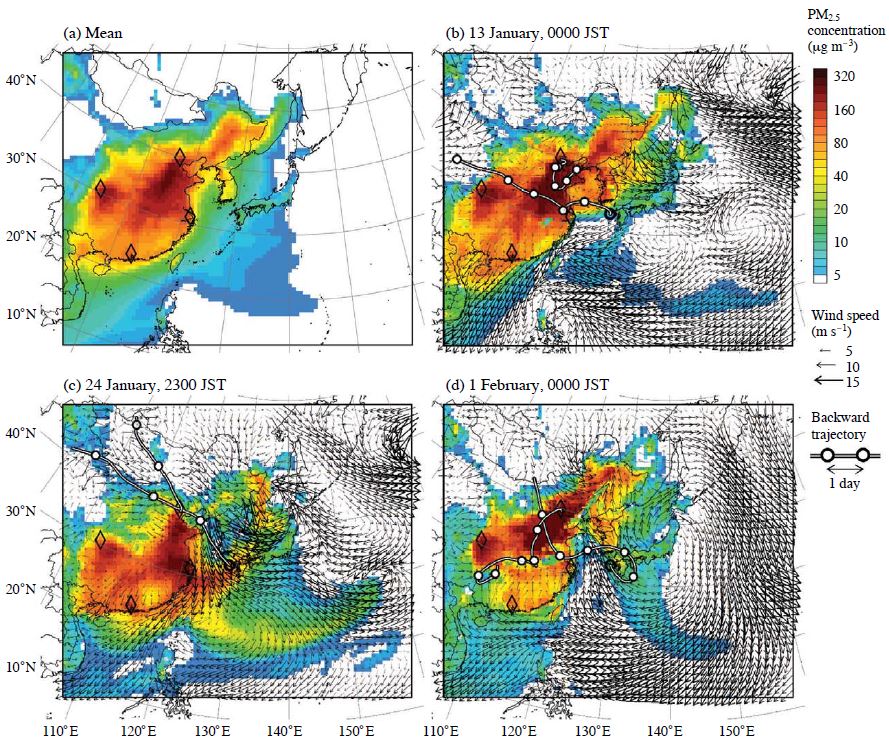
Horizontal distributions of (a) mean PM2.5 concentration from 2 January to 5 February 2013 and hourly PM2.5 concentrations with wind vectors at the first layer and backward trajectories arriving at 300m above Beijing and Fukue at (b) 13 January 2013, 0000 JST, (c) 24 January, 2300 JST and (d) 1 February, 0000 JST.
3. 5 Contribution of Emission Sectors in China to PM2.5 Concentration
Contributions of the four emission sectors in China to PM2.5 concentrations were estimated by conducting five kinds of zero-out emission runs in which emissions from the power generation (EChinaPow0), industry (EChinaInd0), residential (EChinaRes0), transportation (EChinaTra0) sectors or all the four sectors (EChina0) were respectively removed. The contribution rate of each emission sector to PM2.5 concentration is estimated by
| (1) |
The estimated contribution rate of the total emission from the four sectors in China (CRChina) is generally inconsistent with the sum of the estimated contribution rates of the individual sectors (CRChinaPow, CRChinaInd, CRChinaRes and CRChinaTra). The difference is due to the effect of nonlinearity in secondary PM2.5 productions and is defined as
| (2) |
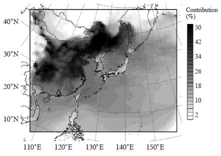
Fig. 6 shows the estimated mean contribution rates of the anthropogenic emissions by sector in China to PM2.5 concentration. The contribution of the total emissions from the four sectors in China accounted for 95% of the mean PM2.5 concentration in the country during the simulation period. The remaining portion was constituted by contributions of initial and boundary conditions, emissions from natural sources, and transport from the other countries. The residential sector had the highest contribution rate, followed by the industrial, power generation and transportation. The order is consistent with that in the amount of primary PM2.5 emissions. The estimated contribution rates of the residential sector were more than 50% at Beijing and Chengdu. Fig. 7 shows a horizontal distribution of the estimated mean contribution rate of the residential emission in China to PM2.5 concentration. The contribution of the residential emission was generally large in cold regions in China. Therefore, large emissions from combustion for heating can cause PM2.5 pollution in the regions. Yonemochi et al. (2013) conducted PM2.5 sampling in Beijing in 9-23 January, 2013. They indicated that emissions from coal combustion for heating should be one of the causes of the extreme PM2.5 pollution, which is consistent with the finding in this study.
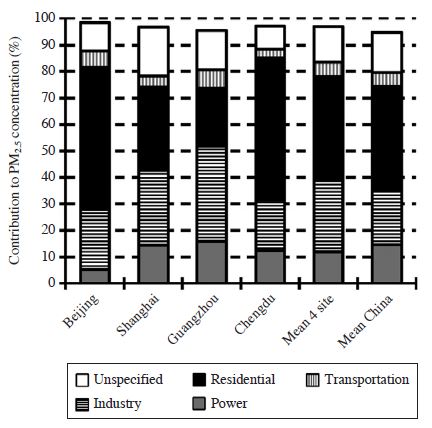
Estimated mean contribution rates of anthropogenic emissions by sector in China to PM2.5 concentration at Beijing, Shanghai, Guangzhou, Chengdu and the four sites, and in the entire area of China in the simulation domain from 2 January to 5 February 2013.
4. CONCLUSIONS
In this study, the extreme PM2.5 pollution in China in winter 2013 was simulated by using the WRF/CMAQ modeling system. The model was run for the period from 1 January to 5 February 2013 in the simulation domain covering East Asia. PM2.5 concentrations in China were generally reproduced by the existing model and input data, including the INTEX-B emission data in the year 2006. Therefore, the extreme PM2.5 pollution seems to be mainly attributed to meteorological (weak wind and stable) conditions rather than emission increases in the past several years. In addition, the model simulated PM2.5 concentrations in Japan as well as China, indicating that the model well captured characteristics of the PM2.5 pollutions in both areas on the windward and leeward sides in East Asia. Note that the model still needs to be revised for better representation of individual PM2.5 components.
The INTEX-B emission data have four sectors: power generation, industry, residential and transportation. Contributions of emissions from the four sectors in China to PM2.5 concentration were estimated by conducting zero-out emission sensitivity runs. The residential sector had the highest contribution rate, followed by the industrial, power generation and transportation. Therefore, the extreme PM2.5 pollution may be also attributed to large primary PM2.5 emissions from combustion for heating in cold regions in China.
Acknowledgments
The observation of PM1 components at Fukue was supported by the Environment Research and Technology Development Fund (B-1006) of the Ministry of the Environment, Japan. We appreciate the U.S embassy in Beijing and consulates in Shanghai, Guangzhou and Chengdu, and the Ministry of Environment in Japan for providing the observation data of PM2.5 concentrations. We are grateful to NMRI and OPRF for providing the ship emission inventories.
References
-
Bey, I., Jacob, D.J., Yantosca, R.M., Logan, J.A., Field, B.D., Fiore, A.M., Li, Q., Liu, H.Y., Mickley, L.J., Schultz, M.G., (2001), Global modeling of tropospheric chemistry with assimilated meteorology: Model description and evaluation, Journal of Geophysical Research D: Atmospheres, 106, p23073-23095.
[https://doi.org/10.1029/2001jd000807]

-
Byun, D.W., Schere, K.L., (2006), Review of the governing equations, computational algorithms, and other components of the Models-3 Community Multiscale Air Quality (CMAQ) modelling system, Applied Mechanics Reviews, 59, p51-77.
[https://doi.org/10.1115/1.2128636]

- Carter, W.P.L., (2000), Implementation of the SAPRC-99 Chemical Mechanism into the Models-3 Framework, Report to the United States Environmental Protection Agency.
-
Chen, F., Dudhia, J., (2001), Coupling an advanced landsurface/hydrology model with the Penn State/NCAR MM5 modeling system. Part I: Model implementation and sensitivity, Monthly Weather Review, 129, p569-585.
[https://doi.org/10.1175/1520-0493(2001)129<0587:CAALSH>2.0.CO;2]

- Draxler, R.R., Hess, G.D., (1997), Description of the Hysplit _4 modeling system, NOAA Tech. Memo, ERL ARL- 224.
-
Duan, F.K., He, K.B., Ma, Y.L., Yang, F.M., Yu, X.C., Cadle, S.H., Chan, T., Mulawa, P.A., (2006), Concentration and chemical characteristics of PM2.5 in Beijing, China: 2001-2002, Science of the Total Environment, 355, p264-275.
[https://doi.org/10.1016/j.scitotenv.2005.03.001]

-
Dudhia, J., (1989), Numerical study of convection observed during the Winter Monsoon Experiment using a mesoscale two-dimensional model, Journal of the Atmospheric Sciences, 46, p3077-3107.
[https://doi.org/10.1175/1520-0469(1989)046<3077:nsocod>2.0.co;2]

-
Emmons, L.K., Walters, S., Hess, P.G., Lamarque, J.-F., Pfister, G.G., Fillmore, D., Granier, C., Guenther, A., Kinnison, D., Laepple, T., Orlando, J., Tie, X., Tyndall, G., Wiedinmyer, C., Baughcum, S.L., Kloster, S., (2010), Description and evaluation of the Model for Ozone and Related chemical Tracers, version 4 (MOZART-4), Geoscientific Model Development, 3, p43-67.
[https://doi.org/10.5194/gmd-3-43-2010]

-
Fu, J.S., Streets, D.G., Jang, C.J., Hao, J., He, K., Wang, L., Zhang, Q., (2009), Modeling regional/urban ozone and particulate matter in Beijing, China, Journal of the Air & Waste Management Association, 59, p37-44.
[https://doi.org/10.3155/1047-3289.59.1.37]

-
Guenther, A., Karl, T., Harley, P., Wiedinmyer, C., Palmer, P.I., Geron, C., (2006), Estimates of global terrestrial isoprene emissions using MEGAN (Model of Emissions of Gases and Aerosols from Nature), Atmospheric Chemistry and Physics, 6, p3181-3210.
[https://doi.org/10.5194/acpd-6-107-2006]

- Hong, S.-Y., Lim, J.-O.J., (2006), The WRF Single-Moment 6-Class Microphysics Scheme (WSM6), Journal of the Korean Meteorological Society, 42, p129-151.
-
Hong, S.-Y., Noh, Y., Dudhia, J., (2006), A new vertical diffusion package with an explicit treatment of entrainment processes, Monthly Weather Review, 134, p2318-2341.
[https://doi.org/10.1175/mwr3199.1]

-
Kain, J.S., (2004), The Kain-Fritsch convective parameterization: An update, Journal of Applied Meteorology, 43, p170-181.
[https://doi.org/10.1175/1520-0450(2004)043<0170:tkcpau>2.0.co;2]

-
Kurokawa, J., Ohara, T., Morikawa, T., Hanayama, S., Janssens-Maenhout, G., Fukui, T., Kawashima, K., Akimoto, H., (2013), Emissions of air pollutants and greenhouse gases over Asian regions during 2000-2008: Regional Emission inventory in ASia (REAS) version 2, Atmospheric Chemistry and Physics, 13, p11019-11058.
[https://doi.org/10.5194/acpd-13-10049-2013]

-
Lin, M., Holloway, T., Carmichael, G.R., Fiore, A.M., (2010), Quantifying pollution inflow and outflow over East Asia in spring with regional and global models, Atmospheric Chemistry and Physics, 10, p4221-4239.
[https://doi.org/10.5194/acp-10-4221-2010]

-
Mlawer, E.J., Taubman, S.J., Brown, P.D., Iacono, M.J., Clough, S.A., (1997), Radiative transfer for inhomogeneous atmospheres: RRTM, a validated correlated-k model for the longwave, Journal of Geophysical Research D: Atmospheres, 102, p16663-16682.
[https://doi.org/10.1029/97jd00237]

- Morikawa, T., Chatani, S., Nakatsuka, S., (2012), Technical report of the Japan Auto-Oil Program: Estimate of emissions from vehicles, Rep. JPEC-2011AQ-02-06, Japan Petroleum Energy Center, Minato-ku, Tokyo, Japan, (in Japanese).
- Nakatsuka, S., Morikawa, T., Chatani, S., Matsunaga, S., (2012), Technical report of the Japan Auto-Oil Program: Estimate of emissions from sectors other than vehicles, Rep. JPEC-2011AQ-02-07, Japan Petroleum Energy Center, Minato-ku, Tokyo, Japan, (in Japanese).
-
Ng, N.L., Herndon, S.C., Trimborn, A., Canagaratna, M.R., Croteau, P.L., Onasch, T.B., Sueper, D., Worsnop, D.R., Zhang, Q., Sun, Y.L., Jayne, J.T., (2011), An Aerosol Chemical Speciation Monitor (ACSM) for routine monitoring of the composition and mass concentrations of ambient aerosol, Aerosol Science and Technology, 45, p770-784.
[https://doi.org/10.1080/02786826.2011.560211]

-
Ohara, T., Akimoto, H., Kurokawa, J., Horii, N., Yamaji, K., Yan, X., Hayasaka, T., (2007), An Asian emission inventory of anthropogenic emission sources for the period 1980-2020, Atmospheric Chemistry and Physics, 7, p4419-4444.
[https://doi.org/10.5194/acp-7-4419-2007]

- OPRF, (2012), Report on the Project for Estimating the Impact of Designation of Emission Control Area on Improvements in Air Quality, Rep. ISBN978-4-88404-282-0, Minato-ku, Tokyo, Japan, (in Japanese).
- Shimadera, H., Hayami, H., Chatani, S., Morino, Y., Mori, Y., Morikawa, T., Yamaji, K., Ohara, T., (2012), Sensitivity analysis of influencing factors on PM2.5 nitrate simulation. paper presented at the 11th Annual CMAS Conference, Chapel Hill, NC, U.S.
- Shimadera, H., Hayami, H., Chatani, S., Morino, Y., Mori, Y., Morikawa, T., Yamaji, K., Ohara, T., (2014), Sensitivity analyses of factors influencing CMAQ performance for fine particulate nitrate, Journal of the Air & Waste Management Association, in press.
-
Shimadera, H., Kondo, A., Kaga, A., Shrestha, K.L., Inoue, Y., (2009), Contribution of transboundary air pollution to ionic concentrations in fog in the Kinki Region of Japan, Atmospheric Environment, 43, p5894-5907.
[https://doi.org/10.1016/j.atmosenv.2009.08.022]

-
Shimadera, H., Kondo, A., Shrestha, K.L., Kaga, A., Inoue, Y., (2011), Annual sulfur deposition through fog, wet and dry deposition in the Kinki Region of Japan, Atmospheric Environment, 45, p6299-6308.
[https://doi.org/10.1016/j.atmosenv.2011.08.055]

-
Skamarock, W.C., Klemp, J.B., (2008), A time-split nonhydrostatic atmospheric model for weather research and forecasting applications, Journal of Computational Physics, 227, p3465-3485.
[https://doi.org/10.1016/j.jcp.2007.01.037]

- Uno, I., Yumimoto, K., Hara, Y., Itahashi, I., Kanaya, Y., Sugimoto, N., Ohara, T., (2013), Why did a remarkably high PM2.5 air pollution occur over China in the winter of 2013?, Journal of Japan Society for Atmospheric Environment, 48, p274-280, (in Japanese).
- WHO, (2006), WHO Air quality guidelines for particulate matter, ozone, nitrogen dioxide and sulfur dioxide. Global update 2005. Summary of risk assessment, Rep. WHO/SDE/PHE/OEH/06.02, Geneva, Switzerland.
- Willmott, C.J., (1981), On the validation of models, Physical Geography, 2, p184-194.
- Yonemochi, S., Chen, X., Miao, P., Lu, S., Oh, K., Umezawa, N., (2013), Characterization of high concentration of PM2.5and PM1collected in Beijing in January, 2013, Journal of Japan Society for Atmospheric Environment, 48, p140-144, (in Japanese).
-
Zhang, Q., Streets, D.G., Carmichael, G.R., He, K., Huo, H., Kannari, A., Klimont, Z., Park, I., Reddy, S., Fu, J.S., Chen, D., Duan, L., Lei, Y., Wang, L., Yao, Z., (2009), Asian emissions in 2006 for the NASA INTEX-B mission, Atmospheric Chemistry and Physics, 9, p5131-5153.
[https://doi.org/10.5194/acpd-9-4081-2009]

-
Zhang, Q., Streets, D.G., He, K., Wang, Y., Richter, A., Burrows, J.P., Uno, I., Jang, C.J., Chen, D., Yao, Z., Lei, Y., (2007), NOXemission trends for China, 1995-2004: The view from the ground and the view from space, Journal of Geophysical Research, 112, pD22306.
[https://doi.org/10.1029/2007jd008684]

-
Zhao, X., Zhang, X., Xu, X., Xu, J., Meng, W., Pu, W., (2009), Seasonal and diurnal variations of ambient PM2.5concentration in urban and rural environments in Beijing, Atmospheric Environment, 43, p2893-2900.
[https://doi.org/10.1016/j.atmosenv.2009.03.009]

- Zhao, P.S., Dong, F., He, D., Zhao, X.J., Zhang, W.Z., Yao, Q., Liu, H.Y., (2013), Characteristics of concentrations and chemical compositions for PM2.5in the region of Beijing, Tianjin, and Hebei, China, Atmospheric Chemistry and Physics, 13, p4631-4644.
- Zheng, M., Salmon, L.G., Schauer, J.J., Zeng, L., Kiang, C.S., Zhang, Y., Cass, G.R., (2005), Seasonal trends in PM2.5source contributions in Beijing, Atmospheric Environment, 39, p3967-3976.

