Source Identification and Estimation of Source Apportionment for Ambient PM₁₀ in Seoul, Korea

2. 1 Sample Collection and Analytical Methods

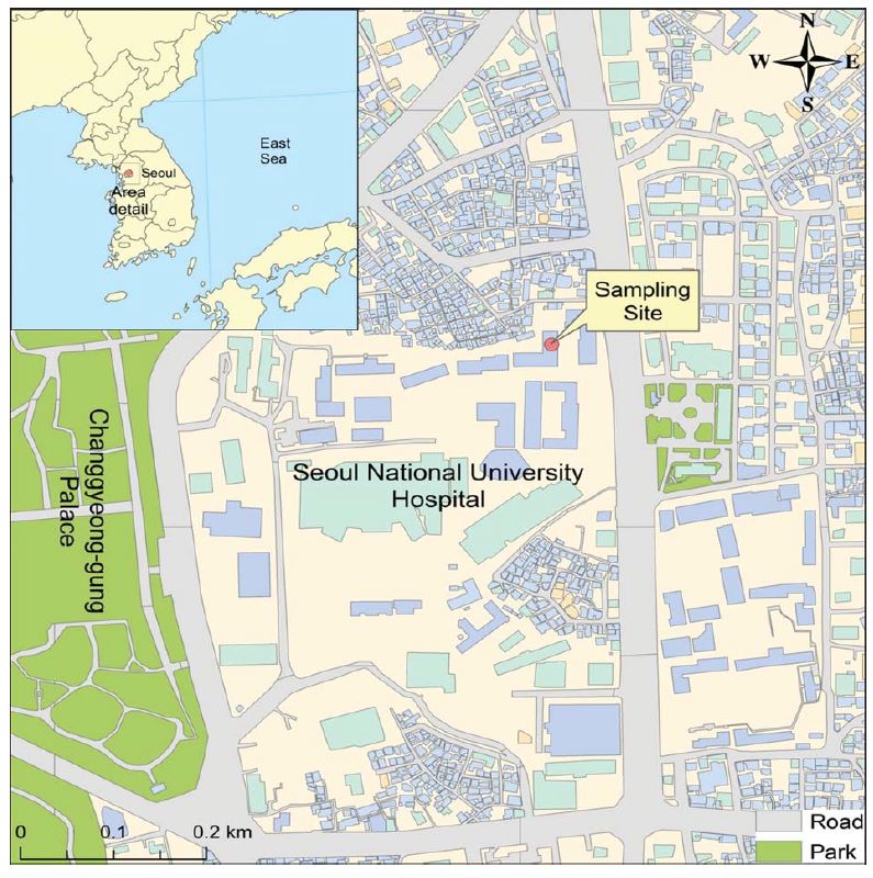
Ambient PM₁₀ samples were collected on the top floor of the School of Public Health building (latitude 37.578, longitude 127.003, and 17 m above ground level) in Seoul National University, Korea (Fig. 1). The land use around the sampling site is mixed commercial and residential area. There are local roads adjacent to the sampling site, which is located about 0.5 km east of the Changgyeong-gung palace.

PM₁₀ samples were collected every 3 days, and a total of 164 samples were collected from August 2006 to November 2007. Samples were collected using three filter packs with PM₁₀ cyclones (URG-2000-30EH, URG). The samples were collected on Teflon, nylon, and quartz filters. The Teflon filters (2.0 μm pore size, Pall Life Science) were used for the analysis of mass concentrations and elemental analysis (a total of 15 elements such as Al, Br, Ca, Cl, Cu, Fe, K, Mg, Mn, Na, Ni, Pb, Si, Ti, and Zn) by particle-induced x-ray emission (PIXE). The nylon filters (1.0 μm pore size, Gelman) were used for the analysis of cations (NH₄ ⁺ and K⁺) and anions (SO₄ ^2- and NO₃ ^-) by ion chromatography (IC). The quartz filters (47 mm, QMA, Whatman) were used for the organic carbon (OC) and elemental carbon (EC) by thermal optical transmittance method (TOT). The detailed analytical methods were reported in a previous study (Heo et al., 2009).

Fig. 1

Location of the sampling site in Seoul metropolitan area.

2. 2 Source Apportionment

PM₁₀ source apportionment was determined using the positive matrix factorization model. This is an advanced factor analysis technique based on a weighted least squares regression and error estimates of the measured data (Paatero, 1997). This model has been widely used in ambient air source apportionment studies (Heo et al., 2013; Lall et al., 2011; Heo et al., 2009; Kim and Hopke, 2007). In this study, the measured concentrations below the method detection limit (MDL) values were replaced by half of the MDL values and their uncertainties were set at five sixths of the MDL values. Missing concentrations were replaced by the geometric mean of the concentrations and their accompanying uncertainties were set at four times the geometric mean concentration (Hwang et al., 2008; Hwang and Hopke, 2006; Polissar et al., 1998).

2. 3 Nonparametric Regression (NPR) Analysis

To identify the impact of local sources from various wind directions, CPF (conditional probability function) and NPR (nonparametric regression) has been used in a number of previous studies (Hwang, 2009; Hwang et al., 2008; Kim and Hopke, 2004; Henry et al., 2002). The NPR model is a regression analysis without parameters, therefore expected values were calculated using source contribution estimates from PMF analysis coupled with the wind direction values measured at the site. The sources are likely to be located in the directions that have high values.

NPR model can be identifying potential locations of the local source with prediction of specific air pollutant concentrations as a function of wind direction and speed. Also, it can be statistically estimate confidence intervals. Predicted concentrations were calculated using the Eq. (1) at θ

Where n is the total number of samples, W_i is the measured wind direction, and C_i is the measured concentration for the ith sample. The average concentration over a sliding window of width Δθ centered at θ is generalized to use Δθ as a smoothing parameter (Henry et al., 2002). If Δθ is too small value, meaningless small peak values will be produced. A Gaussian kernel function, K(x), is used to give different weights to the measurements and defined as Eq. (2).

In this study, the same daily contribution deduced by PMF modelling was assigned to each hour of a given day as C_i in Eq. (1) to match to the hourly wind data and calm winds (<1 m/sec) were excluded from this analysis.

3. 1 Data Analysis

To select the input variables for PMF modeling, the signal-to-noise (S/N) ratios were calculated (Paatero and Hopke, 2003). Variables with very low S/N ratio (≤0.2) were excluded from the PMF analysis, whereas variables with S/N ratio between 0.2 and 2 were downweighted by a factor of 2 or 3. In this study, 21 species (OC, EC, SO₄ ^2-, NO^3-, NH₄ ⁺, Al, Br, Ca, Cl, Cu, Fe, K⁺, K, Mg, Mn, Na, Ni, Pb, Si, Ti, and Zn) were selected for PMF modelling, and the weak variable (Cu) was downweighted. In the case of two bad variables (Br and Ni), these variables were exclude from the PMF analysis in principle due to bad effect for the PMF result. However, these variables were included with adjusted error values because of two variables are important marker species for identification of source. Table 1 shows arithmetic mean, standard deviation, geometric mean, minimum and maximum value, number of BDL, and S/N ratio for individual species during the sampling periods at sampling site.

Table 1.

Summary statistics for the PM10 (μg/m3) and species concentrations (ng/m3) at the sampling site.

3. 2 Determination of the Number of Factors

In order to estimate the optimal number of factors, the mathematical PMF diagnostics was explored. The PMF diagnostics (model error, Q, rotational ambiguity, rotmat, etc.) were based on Lee et al., 1999. In this study, the scaled residual matrix, Q value, and the rotmat matrix (indicates the rotational uncertainty, p×p matrix of standard deviations of rotational coefficients, where p is the number of sources) were used to determine the number of factors. The optimal number of sources was determined to be nine factors based on examination of the scaled residuals and the Q value. In order to explore the rotational freedom, PMF used a parameter, FPEAK, to control the addition and subtraction of the factors. The FPEAK forces PMF to add one g vector to another and to subtract the corresponding f factors from each other, thereby yielding more physically realistic solutions. The Q values were plotted against the FPEAK value to explore the rotational space where only small changes in the Q values are observed. It is also possible to use pairwise scatter plots of the g vectors to help define the FPEAK value (Hwang and Hopke, 2007). In this study, FPEAK values between -1.0 and 1.0 were examined and the value of FPEAK=0.0 provided the most physically meaningful solution.

Also, the parameter FKEY was used to obtain the reasonable source profiles. If specific species in the source profiles do not seem to be realistic based on comparison with measured source profiles and prior analysis of similar data, it is possible to pull values toward zero to obtain the reasonable source profile using the FKEY matrix. The FKEY matrix of integer values has the same dimension as F matrix, where F matrix is a p×m source profile matrix. The details are reported in previous studies (Hwang and Hopke, 2011; Zhao and Hopke, 2004). In this study, values of all elements in the FKEY matrix were set to zero, except for a value of 1 for OC in field burning source.

3. 3 Source Identification and Apportionment

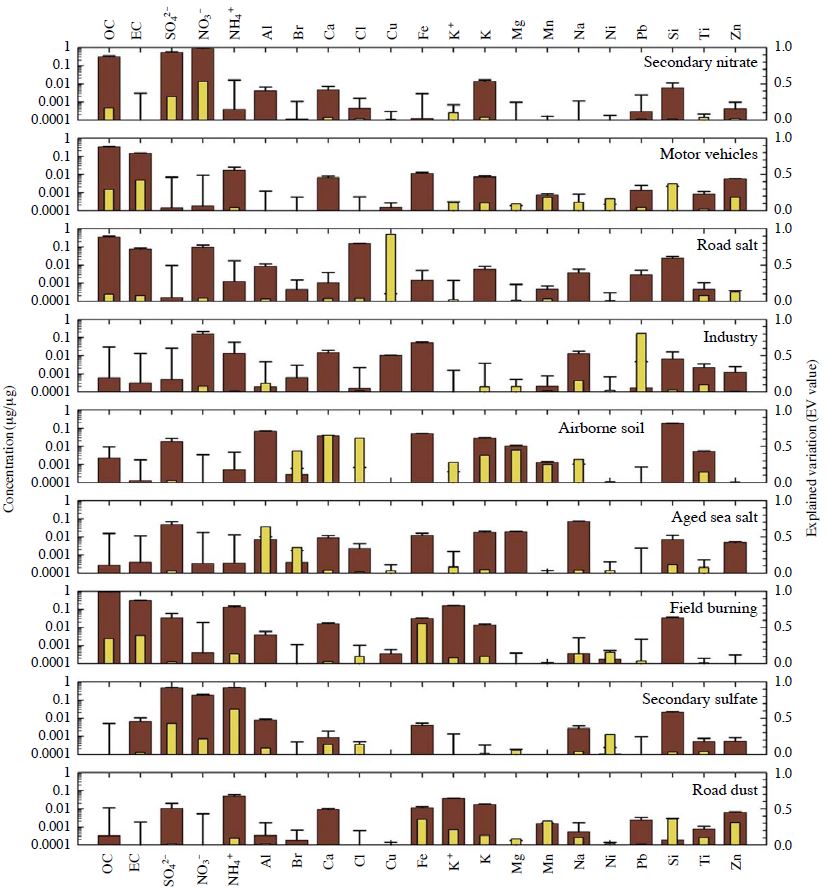
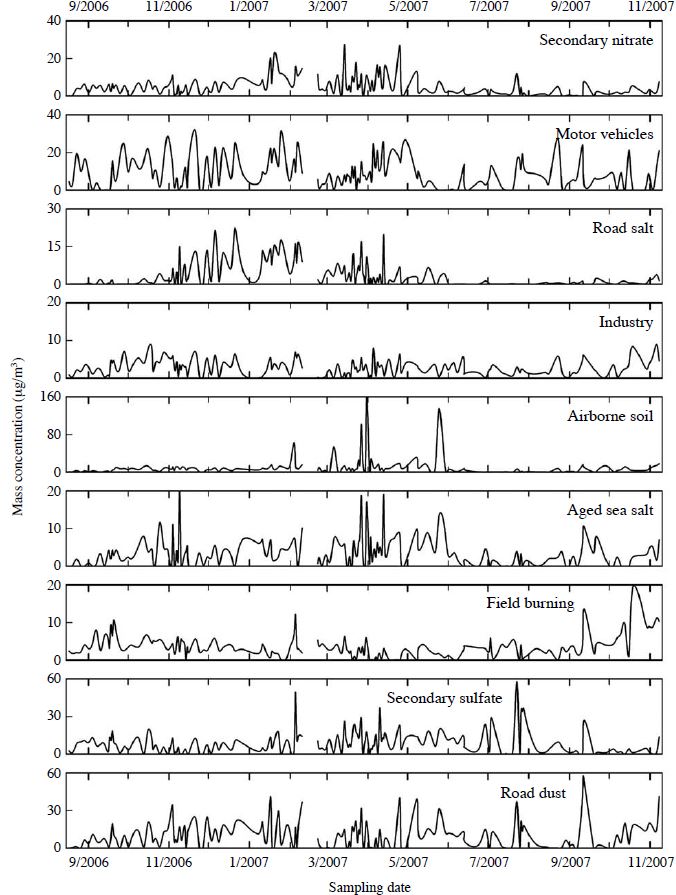
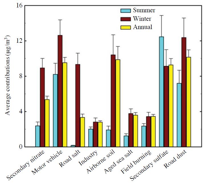
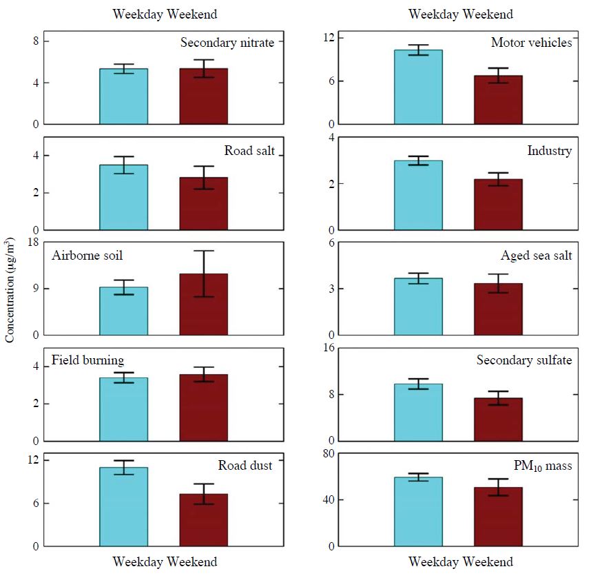
To estimate source apportionment and source profiles in actual units, scaling coefficients were obtained using a multiple linear regression against the measured PM₁₀ mass. Fig. 2 presents the source profiles (value±standard deviation) obtained for the nine factors from the PMF solution at the sampling site in Seoul, where a thin bar denotes explained variation value. Fig. 3 shows the temporal variations of contributions from each source. Table 2 provides a comparison of seasonal contributions for each source and Fig. 4 shows the average source contributions for the whole sampling period. Also, the average source contributions for weekdays and weekend days are presented in Fig. 5.

Fig. 2

Source profiles of the resolved sources measured at the sampling site.

Fig. 3

Temporal variation of source contributions for the sampling site constructed using the PMF model.

Table 2.

Average seasonal source contributions for the sampling site during sampling period.

Fig. 4

Comparison of the average seasonal contributions for each source.

Fig. 5

The average source contributions for weekdays and weekend days at the sampling site.

The species contributing to the first source included NO₃ ^-, SO₄ ^2-, and OC. This profile was identified as secondary nitrate and contributed 9.3% (5.35 μg/m³) to the total PM₁₀ mass concentration. In general, secondary nitrate is known to be seasonal with high contributions in winter season because lower temperatures and high humidity help the formation of secondary nitrate particles (Seinfeld and Pandis, 1998). The seasonal average mass contributions of secondary nitrate show a peak in winter (winter 8.93 μg/m³>spring 7.78 μg/m³>fall 3.44 μg/m³>summer 2.38 μg/m³). To test if the seasonal variation of secondary nitrate is statistically significant, ANOVA was used. There were significant seasonal variations (P value<0.0001) on the contribution of secondary nitrate with spring and winter peaks. The secondary nitrate showed no significant differences in the mean contributions between the weekdays (5.35 μg/m³) and the weekends (5.37 μg/m³) (Fig. 5). The NPR plot for the secondary nitrate source is presented in Fig. 6. This plot indicated secondary nitrate sources located to the west, south, southwest, and north-northeast as shown in Fig. 6.

Fig. 6

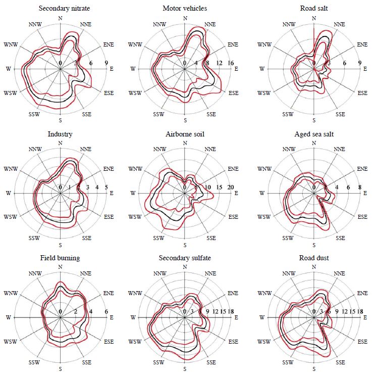
Nonparametric regression (NPR) results based on source contributions obtained by the PMF analysis of data from the sampling site.

The major marker species contributing to the second source profile included OC, EC, Ca, Fe, K, Zn, and Pb, and this profile was classified as motor vehicle source. The two types of motor vehicle sources (i.e. gasoline and diesel emissions) were not separated in this study, though it may be assumed that the contribution of gasoline vehicles is higher than the contribution of diesel vehicles, as land use around the sampling site was mixed commercial and residential, with gasoline engines being far more common than diesel engines. The peak seasonal mass contribution of motor vehicle source was the summer (21.7%, 8.21 μg/m³), the fall (17.7%, 8.64 μg/m³) and winter (17.3%, 12.63 μg/m³) contributions were higher than the spring contribution (13.5%, 9.81 μg/m³). This may be the result of the lower mixedlayer heights in the winter relative to the rest of the year, and thus, a reduced dispersion of these ground level emissions (Hwang and Hopke, 2006). However, in the case of high summer contributions, it will be needed to obtain an understanding of the reason. As shown in Fig. 5, motor vehicle contributions showed higher weekday values (10.35 μg/m³) than those on the weekends (6.78 μg/m³). This result shows that motor vehicle was mainly from vehicles primarily operating in weekdays. The NPR plot indicated motor vehicle sources located to the northeast, southeast, west, and south as shown in Fig. 6 and this results showed good agreement with Heo et al. (2009).

The third source was classified as a road salt source with high abundances of Cl, OC, EC, NO₃ ^-, Si, Al, and Na. The peak seasonal mass contribution of road salt was in the winter (12.8%, 9.33 μg/m³) because road salt released as a deicer on roads in snowfall season. The weekday contribution of road salt was higher than the weekend contribution, similar to the increased contribution of motor vehicles to the weekday samples. Also, the NPR results of road salt showed similar results to the motor vehicle source.

The fourth source was determined to be industry related source. The major species contributing to this source included NO₃ ^-, NH₄ ⁺, Na, Si, Ca, Fe, and Cu. This source contributed 4.9% (2.80 μg/m³) to the total PM₁₀ mass concentration. In the case of this source, the fall contribution (7.1%, 3.44 μg/m³) was higher than other seasonal contributions (winter 3.9%, 2.81 μg/m³; spring 3.4%, 2.48 μg/m³; summer 5.3 %, 2.01vμg/m³). This sampling site is located about 35 km west of a number of industrial complexes (Incheon area) and about 34 km southwest of the Sihwa and Banwol national industrial complexes, which include metal processing, non-ferrous metal smelting, and petroleum chemical process facilities (Gyeonggi-do, 2012). The industry source NPR plot showed good agreement with local source direction, and therefore local industrial activities are likely influence to the industry source of PM₁₀ in sampling area.

The fifth source was identified as airborne soil with high contributions of Si, Al, Fe, K, Ca, Mg, and Ti. The temporal variation of the source contribution plot showed very strong contributions at the end of March, particularly March 27 and 31, 2007 (Fig. 3). It is suggests that the air mass was transported from the Eastern Mongolia and the Gobi Desert and influence of long range transport of Asian dust. Actually, Asian dust episodes have been observed on March 27 and 31, 2007 (KMA, 2007). The peak seasonal mass contribution of airborne soil source was in the spring (27.0%, 19.58 μg/m³).

The sixth source profile was assigned to aged sea salt. The Na and SO₄ ^2-were major species contributing to the aged sea salt source along with minor species such as K, Ca, Mg, and Fe. Although the main species in sea salt are known to be Na, Cl, SO₄ ^2-, K, and Ca (Hopke, 1985), only Na showed a high contribution in association with SO₄ ^2-. The Cl was depleted because NaCl was converted into Na₂SO₄ and NaNO₃as a result of reactions of NaCl with gaseous H₂SO₄ and gaseous HNO₃, respectively (Hwang and Hopke, 2006; Seinfeld and Pandis, 1998). The aged sea salt source peaked in the spring (spring 7.4%, 5.40 μg/m³>fall 6.8%, 3.29 μg/m³>winter 5.2%, 3.77 μg/m³> summer 3.3%, 1.24 μg/m³). This result suggests that the sea salt particles were transported from the Ocean (Yellow Sea) to the west of the site in spring time due to the dominance of wind from the west in the spring time, which is the typical wind direction.

The species associated with the seventh source included OC, EC, SO₄ ^2-, NH₄ ⁺, K⁺, K, Si, Ca, and Fe, and this profile was classified as field burning (included wood combustion and biomass burning) and contributes 6.0% (3.45 μg/m³) to the total PM₁₀ mass concentration. The peak seasonal mass contribution of field burning was the fall (10.8%, 5.27 μg/m³). This source maybe caused by residential wood burning and illegal field burning, such as field burning after harvesting, biofuel burning for heating and cooking, and forest fires that occurred outside of the Seoul area (Heo et al., 2009). There was no significant difference between the concentrations measured on weekdays versus those measured on weekends (Fig. 5).

The eighth source was classified as a secondary sulfate with high abundance of SO₄ ^2-, NH₄ ⁺, and NO₃ ^-, and contributed 16.2% (9.27 μg/m³) to the total PM₁₀ mass concentration. The average seasonal mass contributions show its peak contribution to be in summer (32.9%, 12.46 μg/m³) (Table 2) because formation of secondary sulfate was enhanced by the increased photochemical reaction during the summer time with strong solar intensity. The SO₂ emitted during various combustion processes was converted into H₂SO₄ to form SO₄ ^2- as a result of its photochemical reactions (US EPA, 1999). The NH₄ ⁺ had relatively strong correlations between SO₄ ^2- and NO₃ ^- (0.8 and 0.7), these would presumably exist in the ambient air as secondary aerosols in a sulfate form such as (NH₄)₂SO₄ and (NH₄)₃H(SO₄)₂ as a consequence of homogeneous and heterogeneous reactions (Finlayson-Pitts and Pitts, 2000). As shown in Fig. 6, the NPR plot indicated secondary sulfate source located to the southwest and south. In this area, the largest sources of SO₂ were ships and a coal-fired power plant. In the case of coal-fired power plant, with a production capacity of 4,000 MW, emitted 4485 ton, 5616 ton, 6040 ton of SO₂ during 2005-2007 (KEWP, 2012). Also, the near shore Yellow Sea area where there are active shipping lanes. Many ships burning high sulfur residual oil such that this area can contribute to the secondary sulfate source.

The final source was identified as road dust source. This source profile was similar to the airborne soil source profile, however, these source profiles showed some differences for Zn and Pb. The seasonal average mass contributions of road dust shows a peak in fall (23.1%, 11.27 μg/m³). The seasonal variation of road dust showed similar to the motor vehicle source. This result suggests that road dust particles due to resuspended in the ambient air from operation of motor vehicle.

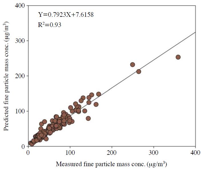
Fig. 7 presents a comparison of the predicted PM₁₀ contributions from all of the identified sources with measured PM₁₀ concentrations. The PMF resolved sources effectively reproduced the measured values (R²=0.93) and account for most of the variation in the PM₁₀ concentrations (slope=0.79).

Fig. 7

Comparison of the predicted total PM10 mass concentrations from the PMF analysis with measured PM10 mass concentrations for the sampling site.

3. 4 Comparison of the Source Apportionment Studies for PM₁₀

In this study, the average contribution of each source was estimated using the PMF model for PM₁₀ in the Seoul, Korea. The source apportionment studies for PM₁₀ were performed beginning of the 1990 in the Korea, therefore reported source apportionment studies for PM₁₀ have been very limited. Several previous studies for the metropolitan area (i.e. Seoul, Gyeonggido, Incheon-si) have identified a total of 10 sources such as fuel combustion (included oil and coal combustion), soil, industry, Fe-related, vehicle (included gasoline and diesel), cement, incinerator, secondary aerosol (included secondary sulfate and secondary nitrate), field burning, and sea salt source, respectively.

Table 3 shows the comparison of PM₁₀ source contributions for the metropolitan area in Korea using the various receptor models. The comparison of source contributions used only identified same sources between this study and previous studies. In the case of soil source contribution for this study, this contribution included contribution of road dust source. The contribution of the soil source was within the range of 16.8 %-35.9%, these results show differences of contribution presumably due to various sampling site, existence of construction works, and inclusion of road dust. The contribution of the industry related source was within range of 3.9%-8.6%, as quite a low contribution to the total PM₁₀ mass concentration, and field burning source contribution showed within range of 7.2%-18.3 %. The contribution of motor vehicle source estimated within range of 7.9%-18.0%. As mentioned above, the KMOE established the “Special Act on Metropolitan Air Quality Improvement” in 2005 in order to improve the PM₁₀ annual concentration in Seoul metropolitan area. It included reduction strategies and management system for vehicle emissions thus vehicle source contributions will be expected lower. Lastly, the contribution of secondary aerosol source estimated within range of 5.1%-17.0%. In particular, in the case of secondary aerosol, the study of the intensive source apportionment for emitted from metropolitan area in Korea and long range transport from China will be the subject of a future study.

Table 3.

Comparison of source contributions (%) for the metropolitan area in Korea using the various receptor models.

References

- Gyeonggi-do, (2012), Industrial Complex Environment Management Office, http://iemo.gg.go.kr.
-
Henry, R.C., Chang, Y.S., Spiegelman, C.H., (2002), Location nearby sources of air pollution by nonparametric regression of atmospheric concentrations on wind direction, Atmospheric Environment, 36, p2237-2244.
[https://doi.org/10.1016/s1352-2310(02)00164-4]
Heo, J.B., Dulger, M., Olson, M.R., McGinnis, J.E., Shelton, B.R., Matsunaga, A., Sioutas, C., Schauer, J.J., (2013), Source apportionments of PM2.5 organic carbon using molecular marker Positive Matrix Factorization and comparison of results from different receptor models, Atmospheric Environment, 73, p51-61.
[https://doi.org/10.1016/j.atmosenv.2013.03.004]
- Heo, J.B., Hopke, P.K., Yi, S.M., (2009), Source apportionment of PM2.5 in Seoul, Korea, Atmos Chem Phys, 9, p4957-4971.
- Hopke, P.K., (1985), Receptor Modeling in Environmental Chemistry, New York, John Willy & Sons.
Hwang, I.J., (2009), Estimation of source apportionment for semi-continuous PM2.5 and identification of location for local point sources at the St. Louis Supersite, USA, Journal of Korean Society for Atmospheric Environment, 25, p154-166, (in Korean).
[https://doi.org/10.5572/kosae.2009.25.2.154]
Hwang, I.J., Hopke, P.K., (2006), Comparison of source apportionments of fine particulate matter at two San Jose Speciation Trends Network sites, Journal of the Air and Waste Management Association, 56, p1287-1300.
[https://doi.org/10.1080/10473289.2006.10464586]
Hwang, I.J., Hopke, P.K., (2007), Estimation of source apportionment and potential source locations of PM2.5 at a west coastal IMPROVE site, Atmospheric Environment, 41, p506-518.
[https://doi.org/10.1016/j.atmosenv.2006.08.043]
Hwang, I.J., Hopke, P.K., (2011), Comparison of source apportionment of PM2.5 using PMF2 and EPA PMF version 2, Asian Journal of Atmospheric Environment, 5, p86-96.
[https://doi.org/10.5572/ajae.2011.5.2.086]
Hwang, I.J., Hopke, P.K., Pinto, J.P., (2008), Source apportionment and spatial distributions of coarse particles during the Regional Air Pollution Study, Environmental Science and Technology, 42, p3524-3530.
[https://doi.org/10.1021/es0716204]
- Hwang, I.J., Kim, D.S., (2003), Estimation of quantitative source contribution of ambient PM10 using the PMF model, Journal of Korean Society for Atmospheric Environment, 19, p719-731, (in Korean).
- KEWP (Korea East-West Power Company), (2011), Korea East-West Power Sustainability Report, KEWP.
Kim, E., Hopke, P.K., (2004), Comparison between Conditional Probability Function and Nonparametric Regression for Fine Particle Source Directions, Atmospheric Environment, 38, p4667-4673.
[https://doi.org/10.1016/j.atmosenv.2004.05.035]
Kim, E., Hopke, P.K., (2007), Source identifications of airborne fine particles using positive matrix factorization and U.S. Environmental Protection Agency positive matrix factorization, Journal of Air and Waste Management Association, 57(7), p811-819.
[https://doi.org/10.3155/1047-3289.57.7.811]
- Kim, K.S., Hwang, I.J., Kim, D.S., (2001), Development of a receptor methodology for quantitative assessment of ambient PM10 sources in Suwon area, Journal of Korean Society for Atmospheric Environment, 17, p119-131, (in korean).
- KMA(Korea Meteorological Administration), (2007), Monthly weather report (March, 2007), KMA, (in korean).
- KMOE (Ministry of Environment, Korea), (2006), White Paper of Environment 2006, KMOE, (in Korean).
Lall, R., Ito, K., Thurston, G.D., (2011), Distributed lag analyses of daily hospital admissions and source-apportioned fine particle air pollution, Environmental Health Perspectives, 119(4), p455-460.
[https://doi.org/10.1289/ehp.1002638]
Lee, E., Chan, C.K., Paatero, P., (1999), Application of positive matrix factorization in source apportionment of particulate pollutants in Hong Kong, Atmospheric Environment, 33(19), p3201-3212.
[https://doi.org/10.1016/s1352-2310(99)00113-2]
- NIER, (2006), Investigation of formation process and establishment of emission reduction strategy for PM10, Korea National Institute of Environmental Research.
Paatero, P., (1997), Least squares formulation of robust nonnegative factor analysis, Chemometrics and Intelligent Laboratory Systems, 37, p23-35.
[https://doi.org/10.1016/s0169-7439(96)00044-5]
Paatero, P., Hopke, P.K., (2003), Discarding or downweighting high-noise variables in factor analytic models, Analytica Chimica Acta, 490, p277-289.
[https://doi.org/10.1016/s0003-2670(02)01643-4]
- Pitts, F.B.J., Pitts, J.N., (2000), Chemistry of the Upper and Lower Atmosphere, San Diego, Academic Press.
Polissar, A.V., Hopke, P.K., Paatero, P., Malm, W.C., Sisler, J.F., (1998), Atmospheric aerosol over Alaska 2. Elemental composition and sources, Journal of Geophysical Research, 103(D15), p19045-19057.
[https://doi.org/10.1029/98jd01212]
- Seinfeld, J.H., Pandis, S.N., (1998), Atmospheric Chemistry and Physics, from Air Pollution to Climate Change, New York, John Wiley & Sons.
- US EPA, (1999), Air quality criteria for particulate matter, I, EPA 600/P-99/002a, Washington, DC.
- Yoo, J.S., Kim, D.S., Kim, Y.S., (1995), Quantitative source estimation of PM-10 in Seoul area, Journal of Korean Air Pollution Research Association, 11, p279-290, (in Korean).
Zhao, W., Hopke, P.K., (2004), Source identification for fine aerosols in Mammoth Cave National Park, Atmospheric Research, 80, p309-322.
[https://doi.org/10.1016/j.atmosres.2005.10.002]