CFD Modeling and Validation of Tracer Gas Dispersion to Evaluate Self-pollution in School Buses
Copyright © 2019 by Asian Journal of Atmospheric Environment
This is an open-access article distributed under the terms of the Creative Commons Attribution Non-Commercial License (http://creativecommons.org/licenses/by-nc/4.0/), which permits unrestricted non-commercial use, distribution, and reproduction in any medium, provided the original work is properly cited.
Abstract
The exhaust gases expelled from the tailpipe during the transit of the buses are composed by different pollutants, each of them dangerous to the human health in different ways. Self-pollution has been detected as a phenomenon related with the passengers exposition to pollutants inside transport buses during their travels. The emissions from the tailpipe make their way to the cabin of the bus, exposing the passengers to toxic gases and particulate matter during the whole time of the trip they are making. The quantitative and detailed modeling of the pollutants in-cabin is important due to the sensitive nature of the children population to respiratory disease related to air pollution. This study assesses self-pollution in school buses using CFD modeling, this is achieved by simulating the dispersion of a tracer gas Sulfur Hexa-Fluoride (SF6) inside and outside the bus. Two previous studies datasets were used to validate the CFD model performance, and accuracy in its capacity to quantitatively describe the phenomenon. The CFD model developed and validated considered the turbulence through the k-epsilon realizable model. The system was considered as a multicomponent single-eulerian-phase flow with the “species to transport” model. Transient formulation and energy were implemented. Mesh was optimized to polyhedral elements, reducing considerably the simulation time by 35%, and mesh size to 25%. The model was able to determine the behavior of the tailpipe emissions and the self-pollution phenomenon into the bus, showing that the highest concentrations (and therefore the maximum exposure) are located in the rear part of the bus. Validation of the CFD results with previous experimental measures and modeling results, reported in two previous studies, determined an error of 12% and 17% for the concentrations outside and inside the bus respectively, correlation coefficient (R2) values between 0.5 and 0.9 were obtained between CFD results for SF6 concentrations and validation dataset.
Keywords:
Air quality modeling, CFD, Self-pollution, Public transport, Tracer gas1. INTRODUCTION
The outflow of exhaust gases generated during the transit of urban-buses is composed by different pollutants products of the combustion in the engine, each of them dangerous to the human health in different ways (Behrentz, 2005; Behrentz et al., 2004). It has been detected that exists a possible self-pollution of this gases in the bus, and that the position of the tailpipe contributes to worsen this issue. One sensitive population exposed to pollution are children that daily use public transport school buses vehicles, exposing them continuously to high pollution levels. The quantitative, and detailed, modeling of the pollutants in-cabin is important due to the sensitive nature of the children population to respiratory disease related to air pollution (Li et al., 2015).
Self-pollution is defined as a portion of the pollutant emissions from the same bus that flow through the windows, or other spaces, to the inside of the vehicle. It has been detected as a phenomenon related with the passengers exposition to pollutants inside transport buses during their travels (Behrentz et al., 2004). The emissions from the tailpipe make their way to the cabin of the bus, exposing the passengers to toxic gases and particulate matter during the whole time of the trip they are making. These emissions can be followed through the injection of a tracer gas, such as Sulfur Hexafluoride (SF6), and directly measuring it inside and outside the cabin of the flow (Li et al., 2015; Behrentz et al., 2004).
This study assesses self-pollution in school buses using Computational Fluid Dynamics (CFD) modeling, this is achieved by simulating, and validating, the dispersion of a tracer gas (SF6) inside and outside the bus (Li et al., 2015; Zhu et al., 2010). Two datasets from previous studies were used to validate the CFD model performance and accuracy in its capacity to quantitatively describe this phenomenon (Li et al., 2015; Behrentz et al., 2004).
The CFD model developed and validated considered the turbulence through the k-epsilon realizable model (Goldberg et al., 1998). The system was considered as a multicomponent single-eulerian-phase flow with “species to transport” model. Transient formulation and energy were implemented (Guevara and Belalcazar, 2017b; Li et al., 2015). Mesh was optimized to polyhedral elements, reducing considerably the simulation time by 35%, and mesh size to 25%. The model was able to determine the behavior of the tailpipe emissions and the self-pollution phenomenon into the bus, showing that the highest concentrations are located in the rear part of the bus, where also the highest exposure of the passengers is evidenced.
Validation of the CFD results with previous experimental measures and CFD modeling results, reported in two previous studies, determined an error of 12% and 17% for the concentrations outside and inside the bus respectively (Behrentz et al., 2004). Correlation coefficient (R) values between 0.7 and 0.9 were obtained between CFD results for SF6 concentrations and validation dataset (Li et al., 2015).
2. MATERIAL AND METHODOLOGY
2. 1 Materials
CFD simulations were performed in a workstation: Intel Xeon 12 core and 16 Gb of RAM. The software used was Ansys Fluent® V19 provided by the Departamento de Ingeniería Química y Ambiental - Universidad Nacional de Colombia.
2. 2 Modeling
CFD modeling was performed based in a finite volume method, 3D geometry of the bus was build using SpaceClaim® (Fig. 1), the geometry was built considering the typical dimensions and design of a school bus (Li et al., 2015), geometry is real-size without scale: approximately 10 meters length, 2.5 meters height and 2.5 meters width. Three positions of the tailpipe were considered; comparison between them allowed to evaluate which tailpipe location has the major impact over the tracer gas concentrations over the bus surface and inside the cabin (self-pollution).

Scholar bus geometry and configuration for CFD modeling: (a) Bus geometry and tailpipe positions, (b) CFD model flow domain.
Extraction of the flow volume as the simulation domain was performed. The domain was discretized into a finite volume element mesh. The mesh initially built for the domain is a non-structured tetrahedral mesh. To ensure the quality of the mesh, the orthogonal quality criteria of the elements was used to reduce the development time that would be required with a mesh convergence analysis; previous studies required big computational power and development time before assuring the best quality mesh. In this study an orthogonal quality of 1×10⁻³ was used as acceptance criteria for the mesh construction.
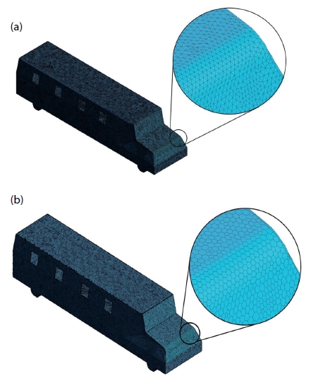
The mesh obtained with this criterion consisted of around 11 million elements, it was after optimized inside Fluent®. This optimization converted the tetrahedral mesh into a polyhedral mesh with around 2.5 million elements (Table 1). The optimized mesh was used in all the simulated cases (Fig. 2).
The CFD model set-up considers the energy transport, turbulence and multicomponent single-eulerian-phase with transient formulation. The transient formulation set-up allows to assess the behavior of the tailpipe gases in time. The multicomponent nature of the system was considered using the species transport model, and the turbulence was modeled with the k-epsilon Realizable turbulence model.
The k-epsilon realizable model considers the flow in motion is free-shear layer and enhances the evaluation of pressure gradients and boundary layer. This turbulence approach allows to simulate strong streamlines with curvatures, vortices and rotation. k-epsilon realizable model also has a better performance for several separated flows and/or flows with complex secondary flow features (The OpenFoam Foundation, 2017; ansys, 2016; Shih et al., 1995).
In the k-epsilon realizable model the term “realizable” means that this alternative model satisfies certain mathematical constraints on the Reynolds stresses, consistent with the physics of turbulent flows. Neither the standard - model nor the RNG - model is realizable (Goldberg et al., 1998).
In this research the k-epsilon realizable model parameters used are summarized in Table 2 (ansys, 2016; Bulat et al., 2013; Tian and Lu, 2013; Goldberg et al., 1998). The parameter values in Table 2 are the standard values commonly used for simulation of uncompressible, turbulent flows. The model constants: C2-epsilon, TKE Prandtl Number and TDR Prandtl Number have been established to ensure that the model performs well for certain canonical flows (ansys, 2016).
The convergence criteria of the CFD model were: scaled residuals and, energy and mass balances. The scaled residuals were set as 1×10⁻⁶ for energy equation, and 1 ×10⁻³ for the other equations. The energy and mass balances were assessed with the criterion of a difference between inlets and outlets lower than 1×10⁻³ kg or W. Relaxation factor used are summarized in Table 3 (ansys, 2016; Guevara Luna, 2003; Versteeg and Malalasekera, 1995).
The simulation strategy planned assumes that there are no other emissions sources different to tailpipe in the system domain, meaning this the gases emitted are the only components dispersed along the flow domain. A major predominance of the wind direction towards the bus due to the forward movement was assumed.
Simulations were performed for 10 seconds clock-time, with a time step of 0.01 seconds based in the Courant Number (Co) criterion (Guevara and Belalcázar, 2017a). The calculation of the Courant Number used the mass velocity in the flow domain (v), the time-step (Δt) and the mesh minimum element size (Δx, 0.015 m for this system).
A Courant Number with a value of 11.1 is lower than 25, the recommended maximum value for the flow simulation to converge (Riaño et al., 2018; Guevara Luna, 2003; Versteeg and Malalasekera, 1995).
A total of five cases where simulated for the three different positions of the tailpipe, three values of bus speed were considered:
- 1. Position 1 at 32 km/h
- 2. Position 1 at 64 km/h
- 3. Position 1 at 100 km/h
- 4. Position 2 at 64 km/h
- 5. Position 3 at 64 km/h
2. 3 Validation
This study has two validation stages, the first stage was to reproduce a first previous study (Li et al., 2015); where the CFD modeling of the tracer gas (SF6) was developed by the authors to reproduce the gas concentration over the outer surface of the bus, these results were compared with the CFD model developed in this study as a first validation step.
The second stage consists in the use of an experimental data measured and reported in a different previous study to be compared against the concentration of the tracer gas (SF6) inside the cabin of the bus obtained from the CFD model developed in the actual study (Behrentz et al., 2004). In this study, the measures were obtained by injection of the tracer gas (SF6) near the end of the tailpipe of the bus and then measured during the transit of the bus under normal conditions. Measurements were made inside and outside the cabin of the bus to determine the exposure of the children to these pollutants.
The two previous research cited were selected for validation of this CFD model development because the same tracer gas (SF6) was used in both, for modeling and measurement.
For the first validating stage, the concentration contours of the tracer gas in the rear surface of the bus are analyzed, this allows qualitatively and quantitatively compare the CFD and experimental contours by defining specific points over such surface.
Values read for the test points in Fig. 3 in both sets of concentration contours allowed to build scatter plots and calculate statistical parameters such as the Pearson Coefficient and R2 to determine the linear relationship between both datasets.
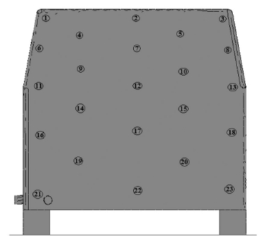
Validation points established for surface tracer gas (SF6) concentration over the rear of the scholar bus.
The second validation stage considers tracer gas (SF6) concentrations inside the bus cabin. The second study recorded tracer gas (SF6) measured data inside and outside school buses, considering different buses models, emissions rates, transit velocities and windows state (open or close). A total of 34 experiments were performed by the authors, but only 3 were selected to validate the CFD model (Table 4). The selected experiments for validation of the CFD model are those which have similar conditions to the CFD model, such as displacement, concentration of SF6, exhaust flowrate and all windows fully opened. With these measured concentrations the error between the CFD model and real on road data is calculated to evaluate the accuracy of the model when assessing the self-pollution phenomenon.
3. RESULTS AND DISCUSSION
3. 1 Model Validation
The results obtained from the CFD simulations for each case are firstly reported as concentration contours of the tracer gas on the rear surface of the bus in ppt.
Regarding the first validation stage, in the Fig. 4 the tracer gas concentration contours is plotted. A similar tendency in both contours, CFD and measured, is observed. This first approach of qualitative analysis is useful to observe that the model reproduces correctly the results from the previous study, however, minimal behavior differences are noted in the contours.
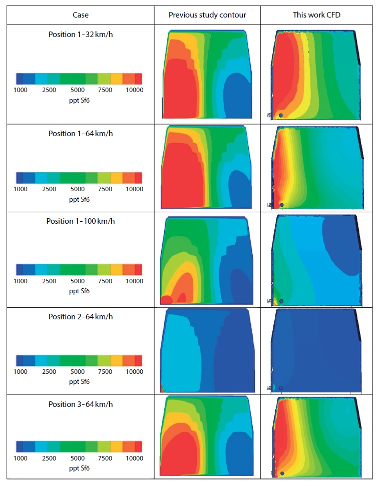
Rear surface tracer gas (SF6) concentration over the scholar bus: Previous study contours and CFD results. For the 5 cases evaluated.
The differences observed between the CFD results from this research and the previous studies can be related to geometry details built for the simulations, the mesh used and the set-up, as the previous study authors did not report the dimensions, the mesh type, elements and quality, nor the setup settings and models of the one they used. Considering this, the assumptions and settings from the setup used in this work CFD model are adequate to study the phenomena of interest.
In both contour sets exist a decreasing tendency in the tracer gas concentration as the velocity increases, this behavior could be explained by the streams and turbulence generated in the air by the transit of the bus, which helps in the dispersion. Dragging in the tracer gas due to the high speed of the air flow that carries along with the emission is evidenced. It is also notorious that there exists a relationship between the tailpipe position and the concentration of the tracer gas, in the positions 1 and 3 is where the highest concentration is detected, whereas for position 2 the proportion of the concentration is down to 10 times less than in the others.
Considering the similitude of the contours between the previous study and this work, a quantitative validation was performed. Graphically the scatter plots represent the accuracy of the CFD model according to the measured data. A linear correlation in these plots allows to determine the relationship between the two datasets; it is desirable that the Pearson coefficient and the R2 values are close to 1.0. As seen in the plots, for each case, R2 values where between 0.5 and 0.9 indicating an accurate performance of the CFD model implemented. However, it is important to consider that for one of the measured data there are several points of the CFD results points, this data pattern affects negatively the correlation in terms of Pearson Coefficient and R2. Nevertheless, it is important to mention that in the results from the previous study, not details such as the tailpipe or wheels were considered; this situation leads to a non-real reproduction of the tracer gas and pollution dispersion evaluated by the previous studies model. The source of error is in this case the previous work results which does not consider details improved in the current development.
The CFD model developed in this research improves the results obtained by previous studies, the accurate consideration of details such as considering the wheels and tailpipes geometry leads to a more realistic representation of the dispersion phenomenon. The avoidance of this details would not be conceptually correct this research aimed to consider as much real features as possible for the geometry involve in the CFD modeling.
The scatter plots from the Fig. 5 show that there exist some values in the X-axis that have multiple corresponding values in the Y-axis, as is shown in the case number 3, this results in a poor correlation (R2=0.5151), however, by reviewing the reference in detail, it is shown that the wheels and tailpipe were not considered in the model, this is a non-real situation due to the inexistence of the wheels in the bus geometry and this affects negatively the model results. In contrast, this study considers the wheels of the bus in the geometry, meshing and CFD simulations, resulting in a more accurate phenomena description and results. By considering the wheels in this study, the final correlation between both studies could achieve higher values.
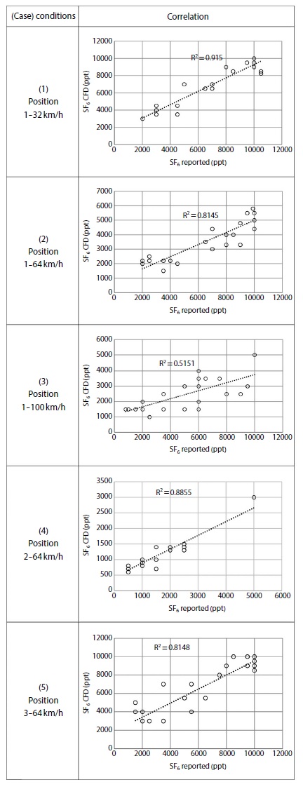
Scatter plots of CFD surface tracer gas (SF6) concentration against reported data from previous study. For the 5 cases evaluated.
To assess the self-pollution inside the bus, comparison of the concentration results obtained from the CFD model with the data measured in the second previous study was the approach. The collected data from this study showed that there is experimentally a quantity of self-pollution inside the bus cabin, this phenomenon is also perceived by the CFD model developed during this research.
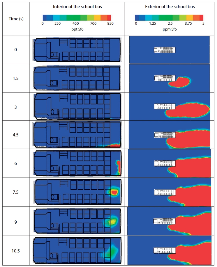
For the assessment of the CFD self-pollution accuracy inside the bus, the results from the CFD model where directly compared with the measurements of the second previous study. The results obtained from the simulations for this case showed a tendency to the infiltration of exhaust gases into the cabin of the bus, these results were obtained through a transient simulation and the contours of the evolution of the concentration of tracer gas (SF6), the contour maps of tracer gas are contained in the Fig. 6. The contours of concentration shown in the left column is the concentration of tracer gas inside the bus in ppt and the contours on the right column is the concentration of tracer gas in the surroundings of the bus in ppm. As the time step advances, according to the transient formulation used, the emission is dispersed behind the bus and this dispersion leads the gases from the tailpipe to the cabin of the bus.
The numerical comparison with the previous study considered data measured inside the buses, three cases of the dataset reported in the study where used to validate in a second stage the results from the CFD model of this research. The concentrations measured inside and outside the bus where averaged and compared with the CFD results. Table 5 show the error between the measured data and the prediction of the CFD model.
The calculated error between CFD and measurement showed that a low level of error is presented by the prediction of the CFD, considering the assumptions made by the model it is an adequate approach to simulate the self-pollution phenomena.
The simulation results allow to determine that the most affected zone inside the bus due to self-pollution is the rear part of the cabin. In the center-rear part of the cabin an accumulation area was identified due to the air flow pattern inside the cabin. However, as the bus advances, the velocity and the exchange of air between the inside and outside of the vehicle, with the windows opened, trend to disperse the gas in the volume of the cabin, notwithstanding, the highest concentrations are in the rear part persists constantly due to the accumulation area identified.
This results leads to identified the rear art of the buses as the more exposed place for children inside scholar buses, and for users of transport systems based in this type of urban buses.
The plume of gases emitted from the tail pipe are dispersed back to the vehicle, and mainly to the left side of the flow domain (Fig. 6). This dispersion pattern evidences an important affectation to other vehicles, and mainly to motorcycles, making passengers of those traffic vehicles to be also exposed to the emission of this medium size buses.
4. CONCLUSIONS
CFD modeling of scholar bus to assess the children’s exposition to self-pollution from the vehicle, considering different cases mainly based in tailpipe positions and vehicle transit velocities, was performed during this research.
The CFD modeling proposed considered in detail the transport phenomena involved in the situation, and the obtained results were validated with tow dataset retrieved from two previous studies (Li et al., 2015; Behrentz et al., 2004). The CFD model was validated obtaining an error of 12% and 17% for the concentrations outside and inside the bus respectively (Behrentz et al., 2004). And a Correlation coefficient (R2) values between 0.5 and 0.9 were obtained between CFD results for SF6 concentrations and validation dataset (Li et al., 2015). Allowing to analyze the spatial and temporal dispersion of pollution at local level using the CFD approach, especially to analyze exposition to self-pollution.
The exposition analysis evidenced the highest concentrations of pollution from the tailpipe is located in the rear-center part of the bus cabin. Meanwhile the outside dispersion of the pollutants emitted from the tailpipe is transported backwards in the flow domain, leading to exposure in other vehicles on road.
Acknowledgments
The authors of this paper would like to thank the financial support from the Universidad Nacional del Colombia to the projects from the Vicedecanatura de Investigación de la Facultad de Ingeniería registered in the HERMES system with QUIPU code number 201010028213 and title “Implementación y validación de un modelo CFD para simular la dispersión de material particulado PM2.5 al interior de buses de transporte público” under the supervision of PhD Luis Carlos Belalcázar and the project from the Vicedecanatura de Investigación de la Facultad de Ingeniería registered in the HERMES system with QUIPU code number 202010027027 and title “Aplicación de la dinámica de fluidos computacional al diseño de reactores químicos” under supervision of PhD. Hugo Galindo for the acquisition of the software license for the development of the simulations.
References
- ansys, (2016), ANSYS Engineering Analysis System User’s Manual (17th ed.), Houston.
-
Behrentz, E., (2005), Vehicle Self-Pollution Intake Fraction: Children’s Exposure to School Bus Emissions, Environmental Science & Technology, 39(8), p2559-2563.
[https://doi.org/10.1021/es040377v]

-
Behrentz, E., Fitz, D.R., Pankratz, D.V., Sabin, L.D., Colome, S.D., Fruin, S.A., Winer, A.M., (2004), Measuring self-pollution in school buses using a tracer gas technique, Atmospheric Environment, 38(23), p3735-3746.
[https://doi.org/10.1016/j.atmosenv.2004.04.007]

-
Bulat, M.P., Bulat, P.V., Tian, C., Lu, Y., Goldberg, U., Peroomian, O., Chakravarthy, S., (2013), Comparison of turbulence models in the calculation of supersonic separated flows, World Applied Sciences Journal, 120(10), p182-192.
[https://doi.org/10.5829/idosi.wasj.2013.27.10.13715]

-
Goldberg, U., Peroomian, O., Chakravarthy, S., (1998), A Wall-Distance-Free k-ε Model With Enhanced Near-Wall Treatment, Journal of Fluids Engineering, 120(3), p457-462.
[https://doi.org/10.1115/1.2820684]

- Guevara Luna, M.A., (2003), Teoría Sobre Modelamiento CFD, Universidad Nacional de Colombia.
- Guevara, M., Belalcázar, L.C., (2017a), NGL supersonic separator: modeling, improvement, and validation and adjustment of k-epsilon RNG modified for swirl flow turbulence model, Revista Facultad de Ingeniería, Universidad de Antioquia, (80), p4-8.
-
Guevara, M., Belalcazar, L., (2017b), NGL supersonic separator: modeling, improvement, and validation and adjustment of k-epsilon RNG modified for swirl flow turbulence model, Revista Facultad de Ingeniería, 82, p82-93.
[https://doi.org/10.17533/udea.redin.n82a11]

-
Li, F., Lee, E.S., Liu, J., Zhu, Y., (2015), Predicting self-pollution inside school buses using a CFD and multi-zone coupled model, Atmospheric Environment, 107, p16-23.
[https://doi.org/10.1016/j.atmosenv.2015.02.024]

- Riaño, S., Guevara Luna, M.A., Belalcázar, L.C., (2018), CFD Modeling and Evaluation of a Bi-STable Micro-Diverter Valve, Ciencia, Tecnologia y Futuro, 8(1), p77-84.
-
Shih, T.-H., Liou, W.W., Shabbir, A., Yang, Z., Zhu, J., (1995), A New k-epsilon Eddy Viscosity For High Reynolds Number Turbulent Flows, Compurers Fluids, 24(3), p227-238.
[https://doi.org/10.1016/0045-7930(94)00032-T]

- The OpenFoam Foundation, (2017), OpenFOAM User Guide V 5.0, Retrieved from http://foam.sourceforge.net/docs/Guides-a4/OpenFOAMUserGuide-A4.pdf.
-
Tian, C., Lu, Y., (2013), Turbulence models of separated flow in shock wave thrust vector nozzle, Engineering Applications of Computational Fluid Mechanics, 7(2), p182-192.
[https://doi.org/10.1080/19942060.2013.11015463]

- Versteeg, H.K., Malalasekera, W., (1995), An Introduction to Computational Fluid Dynamics - The Finite Volume Method. Fluid Flow Handbook, McGraw-Hill, …..
-
Zhu, S., Demokritou, P., Spengler, J., (2010), Experimental and numerical investigation of micro-environmental conditions in public transportation buses, Building and Environment, 45(10), p2077-2088.
[https://doi.org/10.1016/j.buildenv.2010.03.004]


