Performance Evaluation of Four Different Land Surface Models in WRF
Abstract
This study presents a performance evaluation of four different land surface models (LSM) available in Weather Forecast Research (WRF). The research site was located in Haean Basin in South Korea. The basin is very unique by its geomorphology and topography. For a better representation of the complex terrain in the mesoscale model were used a high resolution topography data with a spatial resolution of 30 meters. Additionally, land-use layer was corrected by ground mapping data-sets. The observation equipments used in the study were an ultrasonic anemometer with a gas analyzer, an automatic weather station and a tethered balloon sonde. The model simulation covers a four-day period during autumn. The result shows significant impact of LSM on meteorological simulation. The best agreement between observation and simulation was found in the case of WRF with Noah LSM (WRF-Noah). The WRF with Rapid Update Cycle LSM (WRF-RUC) has a very good agreement with temperature profiles due to successfully predicted fog which appeared during measurements and affected the radiation budget at the basin floor. The WRF with Pleim and Xiu LSM (WRF-PX) and WRF with Thermal Diffusion LSM (WRF-TD) performed insufficiently for simulation of heat fluxes. Both overestimated the sensible and underestimated the latent heat fluxes during the daytime.
Keywords:
Land surface model, WRF, Model evaluation, Surface fluxes, Eddy covariance1. INTRODUCTION
Land-surface processes play an important role in the exchange of heat, moisture, and momentum between the surface and atmosphere. It is important to represent them realistically in Numerical Weather Prediction (NWP) models. Many NWPs use empirical formulas to solve the soil fluxes near the ground surface. The advantage of these techniques is the simplicity and less time consuming computations in NWP. For simulations over complex terrain and simulations of microscale phenomena, more reliable techniques for soil fluxes solution are desirable. For this purpose, several land-surface models (LSM) have been already developed and implemented into mesoscale models (e.g. Chen and Dudhia, 2001; Smirnova et al., 1997; Pielke et al., 1997; Bringfelt, 1996; Pleim and Xiu, 1995; Giorgi et al., 1993; Bougeault et al., 1991).
The LSMs typically compute soil temperature profiles, surface temperature, soil moisture profiles snow cover and canopy properties. Many important land-surface processes are handled in LSMs such as canopy water evapotranspiration, snow evapotranspiration, surface run-off and snow melting, all depending on LSM complexity. LSMs also vary with number of soil and canopy layers. Therefore, each LSM can perform differently. Several comparative studies show that the results of meteorological model are sensitive to the choice of the LSM (e.g. Miao et al., 2007; Singh et al., 2007; Olerud and Sims, 2003). Evaluation of LSMs in NWP help to understand the importance of soil surface processes for further development approaches. On the other hand, the evaluation of the LSMs performance can help NWP model users in LSM selection, if the NWP includes more than one land surface scheme, because the decision can markedly affect the simulation results. This is the main purpose of this paper. A special focus is on simulation in regions with a complex terrain. The 3D meteorological model used for this purpose is Weather Research and Forecasting (WRF) modeling system. Four different LSMs available in version 3.3 were examined for short-time period and compared with the observational data-set. The performance evaluation required a good quality observational data. A continuous and high quality data-set obtained from TERRain and ECOlogical Heterogeneity (TERRECO) campaign fulfilled this requirement.
The TERRECO project is an international cooperation in global change science between Kangwon National University (KNU), the Korean Forest Research Institute (KFRI) and the University of Bayreuth (UBT) in Bavaria, Germany. The project, which is financed by the national research foundations of Germany (DFG) and Korea (KOSEF), extends ongoing research in environmental science at both institutions. The overall goal of the TERRECO project is to understand how expected climate change will influence life in our study areas (http://www.bayceer.uni-bayreuth.de).
2. Model description and experimental design
2. 1 WRF Model Configuration and Initialization
WRF is a next-generation, fully compressible Euler non-hydrostatic mesoscale forecast model with a runtime hydrostatic option. Two cores, Advanced Research WRF (ARW) and Non-hydrostatic Mesoscale Model (NMM), are available in WRF. The WRF-ARW core, used in this study, is based on the Fifth-Generation Penn State/NCAR Mesoscale Model (MM5). The model uses terrain following hydrostatic pressure coordinate system with permitted vertical grid stretching (Laprise, 1992). The horizontal grid in WRF is Arakawa-C grid.
The microphysics scheme used in the simulation is WSM6 that is extension of previous WSM5 scheme. Detailed description of the WSM6 can be found in the work of Hong and Lim (2006). The RRTM longwave and Dudhia shortwave radiation schemes were used in the simulation. The slope inclination and shadow effect by terrain obstacles are considered in the Dudhia’s radiation scheme and used in this study. The vertical sub-grid-scale fluxes were solved using Yonsei University planetary boundary layer (YSU-PBL). More information about YSU-PBL can be found in work of Hong et al. (2006).
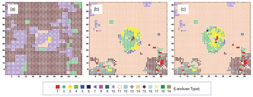
The meteorological initial and boundary conditions for WRF obtained from National Centers for Environmental Prediction (NCEP) are final analysis (FNL) data with 1.0°×1.0° horizontal resolution and 6 hour time interval. The mother domain (D01) used in the simulation has 27 km grid size. The domain is centered at 38°N, 126°E and covers the whole Korean Peninsula, Japan and part of East China (not shown). The horizontal resolutions of D02, D03 and D04 are 9 km, 3 km and 1 km, respectively. The innermost fine domain (D05) is centered at Haean Basin and consists of 54 columns and 57 rows of 0.3×0.3 km grid cells (Fig. 1c). The five domains interact with each other through a twoway nesting strategy. The vertical structure includes 36 layers. Topography and land-use data were interpolated from ASTER Global Digital Elevation Model (ASTER DEM) and Korea Ministry of Environment (KME) with an appropriate spatial resolution for each domain. The KME medium-category land-use classification was used to represent dominant vegetation types (Fig. 2b). Additionally, the KME land-use layer was updated by ground mapping data-sets from TERRECO campaign (Fig. 2c). The rest of regions out of South Korea were filled by United States Geological Survey (USGS) land-use data-set (Fig. 2a).

Design of model domains: (a) Domain D02-D05, (b) domain D04-D05 and (c) domain D05. The location of flux station (triangle) and tethered balloon experiment (cross) are pointed out in the middle of the basin.
2. 2 Land Surface Schemes
The 5-layer thermal diffusion LSM (TD LSM) is based on the 5-layer soil temperature model used in MM5 mesoscale model. The energy budget consists of radiation, sensible and latent heat flux. TD LSM does not predict soil moisture. The soil moisture is fixed with a land-use type and a season dependent constant value. The 5 layers are 1, 2, 4, 8 and 16 cm thick (Skamarock et al., 2008). The model does not have a snow scheme.
The Noah LSM is developed from OSU LSM, described by Chen and Dudhia (2001). The model includes diurnal dependent Penman potential evaporation (Mahrt and Pan, 1984), multilayer soil model of Mahrt and Pan (1984) and canopy model of Pan and Mahrt (1987). The LSM predicts soil moisture and temperature in 4 layers. The layer thickness is 10, 30, 60 and 100 cm from top to bottom. The model is able to predict canopy moisture, water-equivalent snow depth and soil ice (Skamarock et al., 2008).
The Rapid Update Cycle LSM (RUC LSM) includes multilevel soil model with 6 default levels. The number of levels can be increased. The model solves heat diffusion, Richards diffusive and gravitational motions for soil moisture transfer (Richards, 1931). In the cold season phase changes of soil moisture are considered (Smirnova et al., 1997). Special feature of RUC LSM is a thin layer spanning the ground surface that includes half of the first atmospheric layer and half of the top soil layer is used to solve the energy budgets. The heat storage in the layer is determined by contribution of soil fluxes and atmospheric fluxes (Smirnova et al., 1997). In RUC LSM, the latent heat flux is directly affected by vegetation through incorporation of free water from canopy and evapotranspiration. The vegetation processes are treated similarly to Noah LSM following concept developed by Pan and Mahrt (1987).
The Pleim and Xiu LSM is based on a set of five partial differential equations for soil temperature and soil moisture in two layers (1-cm surface layer and 1-m root zone layer) and canopy moisture (Pleim and Xiu, 1995).
2. 3 Observation
The research site was located in Haean Catchment, Kangwon province, South Korea. Haean is an intensively used agricultural region surrounded by forested mountains. The dominant crop types in Haean are rice paddy, radish, bean and potato.
Basic meteorological variables were observed at 2.5 m above ground level with an Automatic Weather Station (AWS, WS-GP1, Delta-T Devices Ltd., UK) located at a rice field (38°17ʹ27ʺ N, 128°07ʹ50ʺ E, 457 m a.s.l.). Measured variables include air temperature, wind speed, wind direction, relative humidity, precipitation, and global radiation.
Located close to the AWS an eddy-covariance measurement system (38°17ʹ28ʺ N, 128°07ʹ52ʺ E) was installed on a 2-m-high mast, to obtain the turbulent atmospheric fluxes of sensible and latent heat and carbon dioxide (CO2). The system was equipped with an ultrasonic anemometer (USA-1, Meteorologische Messtechnik GmbH, Germany) and a fast-response openpath H2O/CO2 gas analyzer (LI-7500, LI-COR Inc., USA) both working at a sampling frequency of 20 Hz. The eddy-covariance software package TK3 (Mauder and Foken, 2011), developed by the Department of Micrometeorology, University of Bayreuth, post-processed the high-frequency raw data according to all international agreed procedures. As result correct 30-minute aggregated sensible and latent heat and CO2 fluxes are available. The detailed calculating and correcting strategy of TK3 could be found in Mauder and Foken (2011) and Foken et al. (2012).
The period from Sep. 23 to 26 (DOY 266 to 269), 2010, was picked out as Golden Days for the validation of models. During this period it was either sunny or cloudy with radiation fog events in the morning. The rice paddies were in the late growing season before harvest with a canopy height of 0.88 m and a leaf area index of 0.68 m2 m-2. The field was irrigated with a water depth of 2 cm. For further information about the field observation, see Zhao et al. (2011).
A multi-step outlier check procedure (Zhao and Lüers, 2012) was applied on both meteorological variables and turbulence fluxes to ensure the high quality of data. as an enhanced quality control procedure. Briefly speaking, this procedure filters those data as outliers that fall beyond the physical thresholds, or have poor quality flags (Foken et al., 2004; Foken and Wichura, 1996), or occur during a bad instrument status, or fail in the statistical check. A quality-controlled data-set is used for the validation of the models.
Tethered balloon soundings were performed from the basin floor during clear undisturbed nights on 24th and 25th of September 2010 (Fig. 1). Since the Haean basin is very close to the demilitarized zone between North and South Korea any radio signal based data transmission was forbidden. Therefore, instead of common radio-sonde, a lightweight probe with internal memory and consisting of temperature/humidity sensor and pressure sensor was used.
3. Results and discussion
3. 1 Temperature
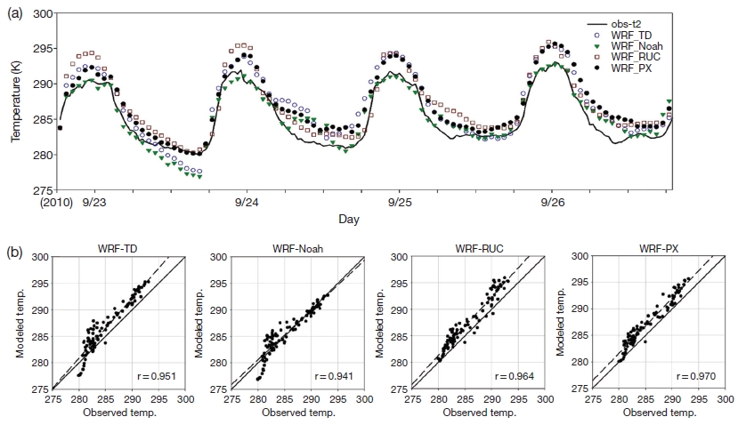
The modeled near surface temperatures (at 2 m above surface) were compared with the measured in Fig. 3. All four models performed quite well with IA higher than 0.9. The best results were given by WRF-Noah with the highest IA (0.95) and lowest MB (0.29°K) (Table 1). Significantly underestimated temperature can be seen in the early morning on 24th of September when the maximal temperature difference between the predicted and observed temperature reached 3.15°K. Similar temperature drop was produced by WRF-TD (Fig. 3a) and the maximal difference reached 2.8°K. Another significant deviation produced by WRF-Noah was on 24th September at night. The model overestimated the temperature by 3.4 K. The low RMSE (0.089) indicates that both errors are obviously non-systematic and except these two deviations the WRF-Noah performed sufficiently. Other models tended to overestimate the temperature especially during the daytime periods. This is most evident in case of WRF-RUC. All models (including WRF-Noah) seem to be skeptic to nocturnal cooling during the first half of nights.
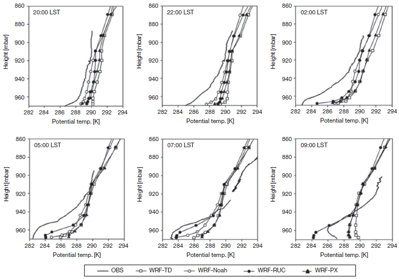
The potential temperature profiles were compared with tethered balloon soundings. The underestimated nocturnal cooling can be seen in the potential temperature profiles as well (Fig. 4). At 20:00, the most realistic simulation seems WRF-Noah. However, the profile does not change much between 22:00 and 02:00. An interesting finding was, the successful prediction of the fog layer formation using WRF-RUC which might be related to the overestimated evaporation expressed as latent heat energy flux in Fig. 6. The overestimated evaporation compensates the radiative cooling deficit (Fig. 3) and allows the saturation in lower model’s layers. The shading effect of fog layer is then well simulated and the profiles of potential temperatures are in closer agreement with the observation (Fig. 5). This can be very well seen in Fig. 4 at 9:00 when the WRFRUC follows the temperature inversion in the fog layer while other WRF-LSMs already predicted the well mixed layer.
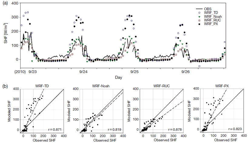
(a) Comparison of Observed and modeled hourly sensible heat fluxes. (b) relation between observed and modeled values for four WRF-LSMs.
3. 2 Surface Energy Fluxes
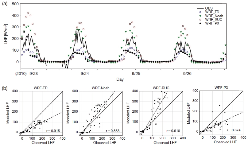
The sensible (SHF) and latent heat fluxes (LHF) are compared with measured fluxes in Fig. 5. and Fig. 6. The gaps of LHF, during night time are caused by the bad working condition when water droplets condensed on the light path of the gas analyzer during fog events.
The modeled heat fluxes by WRF-TD and WRF-PX are very similar. Both of them significantly overestimated SHF and underestimated LHF during the day time. The WRF-TD has the highest RMSE among all models for SHF (Table 1). Better agreement is found between predicted and measured SHF for WRF-RUC and WRF-Noah. The WRF-RUC underestimated the SHF during the day time, although smaller RMSE (28.19) was found compare to WRF-Noah (33.15). For LHF the WRF-Noah showed best results with slight overestimation. The RMSE of WRF-Noah is higher than WRF-TD, but small RMSEs indicates that this was caused by non-systematic error. On other hand WRFTD has greater RMSEs compare to RMSEu and underestimated the LHF continuously. The second best IA was given by WRF-RUC but it also produced the greatest RMSE (89.28) and positive MB (51.7 W m-2). The overestimation is evident during the noon and the maximal LHF.
4. Summary and Conclusion
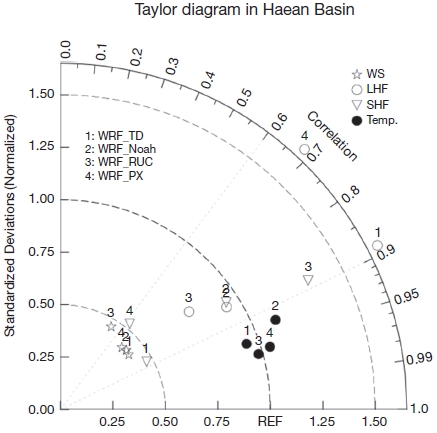
In this research we statistically evaluated four land surface schemes available in 3D WRF 3.3 model against observational data. To provide a concise statistical summary the results are plotted in Taylor diagram (Fig. 7). The best performance for our study case shows WRFNoah. The model very well predicts the near surface temperature and produced best results for LHF. WRF-RUC performed quit well, but SHF tends to underestimate the daytime SHF and overestimate LHF. The fact that WRF-RUC was very accurate during late evenings, indicates that the model might suits well in terms of surface fluxes for simulations of stable atmospheric condition. The remaining WRF-TD and WRF-PX show very similar heat fluxes results and performed insufficiently in our study case. Both tends to significantly overestimates SHF and underestimate LHF almost twice. The TD-LSM is quite old scheme without any moisture prediction, therefore the usage is currently very rare. In case of PX-LSM another study with combining of several physics schemes such a PX PBL would be desirable. The near surface temperature was in good agreement for all tested models. Since the simulation was performed only for clear sky day, an evaluation of the LSMs performance under different weather conditions is desirable.
Acknowledgments
We deeply appreciate Prof. Dr. Thomas Foken, Head of the Department of Micrometeorology, University of Bayreuth, for his helpful comments. We thank Prof. Dr. John Tenhunen, Chair of the Department of Plant Ecology, University of Bayreuth, for his great support. We are also thankful to Dr. Andrei Serafimovich who provided us many comments. This study was carried out as part of the International Research Training Group TERRECO (GRK 1565/1) funded by the Deutsche Forschungsgemeinschaft (DFG) at the University of Bayreuth, Germany and the Korean Research Foundation (KRF) at Kangwon National University, Chuncheon, South Korea. The first author was supported by the KNU (Grant No. C1009653-01-01).
REFERENCES
-
Bougeault, P., Noilhan, J., Lacarrere, P., Mascart, P., (1991), An experiment with an advanced surface parameterization in a mesobeta-scale model. Part I: Implementation, Monthly Weather Review, 119, p2358-2373.
[https://doi.org/10.1175/1520-0493(1991)119<2358:aewaas>2.0.co;2]

- Bringfelt, B., (1996), Tests of a new land surface treatment in HIRLAM. HIRLAM Tech. Rep. 23, Swedish Meteorological and Hydrological Institute, Norrkuping, Sweden, p72.
- Chen, F., Dudhia, J., (2001), Coupling an advance land surface-hydrology model with the Penn State-NCAR MM5 modeling system: Model implementation an sensitivity, Monthly Weather Review, 129, p569-585.
- Foken, T., Göckede, M., Mauder, M., Mahrt, L., Amiro, B.D., Munger, J.W., (2004), Post-field data quality control, Handbook of micrometeorology, p181-208.
-
Foken, T., Leuning, R., Oncley, S.R., Mauder, M., Aubinet, M., (2012), Corrections and Data Quality Control, in Eddy Covariance M. Aubinet edited by, T. Vesala, and D. Papale, p85-131, Springer, Netherlands.
[https://doi.org/10.1007/978-94-007-2351-1_4]

-
Foken, T., Wichura, B., (1996), Tools for quality assessment of surface-based flux measurements, Agricultural and Forest Meteorology, 78(1-2), p83-105.
[https://doi.org/10.1016/0168-1923(95)02248-1]

-
Giorgi, F., Marinucci, M.R., Bates, G., (1993), Development of a second-generation regional climate model (RegCM2). Part II: Convective processes and assimilation of lateral boundary conditions, Monthly Weather Review, 121, p2814-2832.
[https://doi.org/10.1175/1520-0493(1993)121<2814:doasgr>2.0.co;2]

- Hong, S., Lim, J.J., (2006), The WRF Single-Moment 6-Class Microphysics Scheme (WSM6), Journal of the Korean Meteorological Society, 42(2), p129-151.
-
Hong, S.-Y., Noh, Y., Dudhia, J., (2006), A new vertical diffusion package with an explicit treatment of entrainment processes, Monthly Weather Review, 134, p2318-2341.
[https://doi.org/10.1175/mwr3199.1]

-
Laprise, R., (1992), The Euler Equations of motion with hydrostatic pressure as as independent variable, Monthly Weather Review, 120, p197-207.
[https://doi.org/10.1175/1520-0493(1992)120<0197:teeomw>2.0.co;2]

-
Mahrt, L., Ek, M., (1984), The influence of atmospheric stability on potential evaporation, Journal of Climate and Applied Meteorology, 23, p222-234.
[https://doi.org/10.1175/1520-0450(1984)023<0222:tioaso>2.0.co;2]

- Mauder, M., Foken, T., (2011), Documentation and instruction manual of the eddy covariance soft-ware package TK3, Universität Bayreuth, Abt. Mikrometeorologie, Print, ISSN 1614-8916, Arbeitsergebnisse 46.
- Miao, J.-F., Chen, D., Borne, K., (2007), Evaluation and Comparison of Noah and Pleim-Xiu Land Surface Models in MM5 Using GOTE2001 Data : Spatial and Temparal Variations in Near-Surface Air Temperature, Journal of Applied Meteorology and Climatology, 46, p1587-1605.
- Olerud, D., Sims, A. cited, (2003), MM5 sensitivity modeling in support of VISTAS (Visibility Improvement-State and Tribal Association): Task 2e deliverable.
- Pan, H.-L., Mahrt, L., (1987), Interaction between soil hydrology and boundary-layer development, Boundary-Layer Meteorology, 388, p185-202.
-
Pielke, R.A., Lee, T.J., Copeland, J.H., Eastman, J.L., Ziegler, C.L., Finley, C.A., (1997), Use of USGS-provided data to improve weather and climate simulations, Ecological Applications, 7, p3-21.
[https://doi.org/10.2307/2269403]

-
Pleim, J.E., Xiu, A., (1995), Development and testing of a surface flux and planetary boundary layer model for application in mesoscale models, Journal of Applied Meteorology, 34, p16-32.
[https://doi.org/10.1175/1520-0450-34.1.16]

-
Richards, L.A., (1931), Capillary conduction of liquids through porous mediums, Physics, 1, p318-333.
[https://doi.org/10.1063/1.1745010]

-
Singh, A.P., Mohanty, U.C., Sinha, P., Mandal, M., (2007), Influence of different land-surface processes on Indian summer monsoon circulation, Natural Hazards, 42, p423-438.
[https://doi.org/10.1007/s11069-006-9079-9]

- Skamarock, W.C. Coauthors, (2008), A Description of the Advanced Research WRF Version 3, NCAR technical note, NCAR/TN-475+STR.
- Smirnova, T.G., Brown, J.M., Benjamin, S.G., Kim, D., (1997), Parameterization of cold-season processes in the MAPS land-surface scheme, Monthly Weather Review, 128, p1870-1884.
- Willmott, C., (1981), On the Validation of models, Physical Geography, 2, p183-194.
-
Zhao, P., Lüers, J., (2012), Improved determination of daytime net ecosystem exchange of carbon dioxide at croplands, Biogeosciences Discussions, 9(3), p2883-2919.
[https://doi.org/10.5194/bgd-9-2883-2012]

- Zhao, P., Lüers, J., Olesch, J., Foken, T., (2011), Documentation of the observation period, May 12th to Nov. 8th, 2010, Haean, South Korea, Universität Bayreuth, Abt. Mikrometeorologie, Print, ISSN 1614-8916, Arbeitsergebnisse 45.
Appendix
Appendix.
Several statistical variables have been computed to evaluate the performance of WRF-LSMs.
The Index of Agreement (IA) presented by Willmott (1981) as an alternative to r and r2 (coefficient of determination) reflects the degree to which model’s simulations are error free. IA can be obtained from:
| (1) |
Where, Pi and Oi are predicted and observed values, respectively. The actual size of error produced by the model was obtained by estimation of root mean square error (RMSE),
| (2) |
Since the RMSE does not illuminate the source or type of error the systematic RMSE (RMSEs) and un-systematic RMSE (RMSEu) were calculated as well:
| (3) |
| (4) |
where P* is given by:
| (5) |
and a, b are the coefficients of an ordinary least-squares.
The mean bias is generally defined as
| (6) |
Additionally, fractional bias screening test was performed. The fractional bias is given by:
| (7) |
where and are the averages of predicted and observed values.
